4. The statistical data of an urban spot speed study is given below. A set of 130 observations of spot speeds made by timing vehicles through a "Trap" of 88ft. The stopwatch was used to obtain data. The stopwatch data are grouped into 0.2 sec. Classes. The first column of the table shows the midpoint of each group. The second column of the table shows the frequency of the observations. Compute the following statistical values. a) The speed of each time class in mph (show it in the third column) b) The cumulative percent of vehicles traveling at or below indicated speed shown in the third column in mph (show it in the forth column) c) Mean or average speed (time-mean speed), median, mode, standard deviation, standard error of the mean, average time, space-mean speed, variance, 15%, and 85% speed. d) Plot the cumulative percentage, and show the statistical values of item (c) on the graph. e) Plot the frequency distribution curve and show the statistical values on the graph.
4. The statistical data of an urban spot speed study is given below. A set of 130 observations of spot speeds made by timing vehicles through a "Trap" of 88ft. The stopwatch was used to obtain data. The stopwatch data are grouped into 0.2 sec. Classes. The first column of the table shows the midpoint of each group. The second column of the table shows the frequency of the observations. Compute the following statistical values. a) The speed of each time class in mph (show it in the third column) b) The cumulative percent of vehicles traveling at or below indicated speed shown in the third column in mph (show it in the forth column) c) Mean or average speed (time-mean speed), median, mode, standard deviation, standard error of the mean, average time, space-mean speed, variance, 15%, and 85% speed. d) Plot the cumulative percentage, and show the statistical values of item (c) on the graph. e) Plot the frequency distribution curve and show the statistical values on the graph.

Traffic and Highway Engineering
5th Edition
ISBN:9781305156241
Author:Garber, Nicholas J.
Publisher:Garber, Nicholas J.
Chapter4: Traffic Engineering Studies
Section: Chapter Questions
Problem 3P

Related questions

Question
Transcribed Image Text:4. The statistical data of an urban spot speed study is given below. A set of 130 observations of
spot speeds made by timing vehicles through a "Trap" of 88ft. The stopwatch was used to obtain
data. The stopwatch data are grouped into 0.2 sec. Classes. The first column of the table shows
the midpoint of each group.
The second column of the table shows the frequency of the
observations. Compute the following statistical values.
a) The speed of each time class in mph (show it in the third column)
b) The cumulative percent of vehicles traveling at or below indicated speed shown in the
third column in mph (show it in the forth column)
c) Mean or average speed (time-mean speed), median, mode, standard deviation, standard
error of the mean, average time, space-mean speed, variance, 15%, and 85% speed.
d) Plot the cumulative percentage, and show the statistical values of item (c) on the graph.
e) Plot the frequency distribution curve and show the statistical values on the graph.
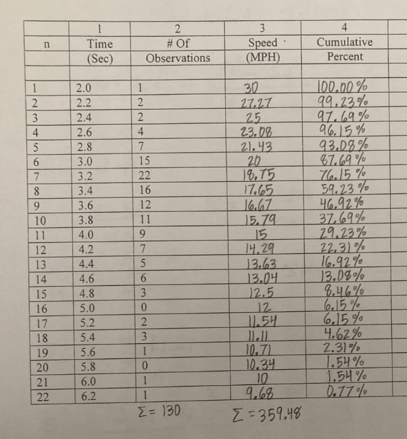
Transcribed Image Text:1
2
3
4
n
Time
# Of
Speed
Cumulative
(Sec)
Observations
(MPH)
Percent
1
2.0
1
30
100.00%
23456789
2.2
2.4
2.6
224
2
27.27
99.23%
2
25
97.69%
23.08
96.15%
2.8
7
21.43
93.08%
3.0
15
20
87.69%
3.2
22
18.75
76.15%
3.4
16
17.65
59.23%
9
3.6
12
16.67
46.92%
10
3.8
11
15.79
37.69%
11
4.0
9
15
29.23%
12
4.2
7
14.29
22.31%
13
14
34
4.4
5
13.63
16.92%
4.6
6
13.04
13.08%
15
4.8
3
12.5
8.46%
16
17
67
5.0
0
12
6.15%
5.2
2
11.54
6.15%
18
5.4
3
11.11
4.62%
19
5.6
1
10.71
2.31%
20
5.8
0
10.34
1.54%
21
6.0
1
10
1.54%
22
6.2
1
9.68
0.77%
Σ= 130
Z=359.48
Expert Solution
This question has been solved!
Explore an expertly crafted, step-by-step solution for a thorough understanding of key concepts.

This is a popular solution!

Trending now
This is a popular solution!

Step by step
Solved in 7 steps with 6 images

Knowledge Booster


Learn more about
Need a deep-dive on the concept behind this application? Look no further. Learn more about this topic, civil-engineering and related others by exploring similar questions and additional content below.Recommended textbooks for you
Traffic and Highway Engineering
Civil Engineering
ISBN:
9781305156241
Author:
Garber, Nicholas J.
Publisher:
Cengage Learning
Traffic and Highway Engineering
Civil Engineering
ISBN:
9781305156241
Author:
Garber, Nicholas J.
Publisher:
Cengage Learning