4.32 Investment risk analysis. The risk of a portfolio of financial assets is sometimes called investment risk. In general, in- vestment risk is typically measured by computing the vari- ance or standard deviation of the probability distribution that describes the decision maker's potential outcomes (gains or losses). The greater the variation in potential outcomes, the greater the uncertainty faced by the decision maker; the smaller the variation in potential outcomes, the more predictable the decision maker's gains or losses. The two discrete probability distributions given in the next table were developed from historical data. They describe the potential total physical damage losses next year to the fleets of delivery trucks of two different firms. Loss Next Year $0 500 NW 1,000 1,500 2,000 2,500 Firm A 3,000 3,500 4,000 4,500 5,000 Firm B Probability Loss Next Year $0 200 .01 .01 35 .30 .02 .01 .01 .01 700 1,200 1,700 2,200 2,700 3,200 3,700 4,200 4,700 Probability 00 .01 .02 .30 .30 .02 01 a. Verify that both firms have the same expected total physical damage loss. b. Compute the standard deviation of each prob- ability distribution and determine which firm faces the greater risk of physical damage to its fleet next
4.32 Investment risk analysis. The risk of a portfolio of financial assets is sometimes called investment risk. In general, in- vestment risk is typically measured by computing the vari- ance or standard deviation of the probability distribution that describes the decision maker's potential outcomes (gains or losses). The greater the variation in potential outcomes, the greater the uncertainty faced by the decision maker; the smaller the variation in potential outcomes, the more predictable the decision maker's gains or losses. The two discrete probability distributions given in the next table were developed from historical data. They describe the potential total physical damage losses next year to the fleets of delivery trucks of two different firms. Loss Next Year $0 500 NW 1,000 1,500 2,000 2,500 Firm A 3,000 3,500 4,000 4,500 5,000 Firm B Probability Loss Next Year $0 200 .01 .01 35 .30 .02 .01 .01 .01 700 1,200 1,700 2,200 2,700 3,200 3,700 4,200 4,700 Probability 00 .01 .02 .30 .30 .02 01 a. Verify that both firms have the same expected total physical damage loss. b. Compute the standard deviation of each prob- ability distribution and determine which firm faces the greater risk of physical damage to its fleet next

Chapter8: Analysis Of Risk And Return
Section: Chapter Questions
Problem 13QTD

Related questions

Question
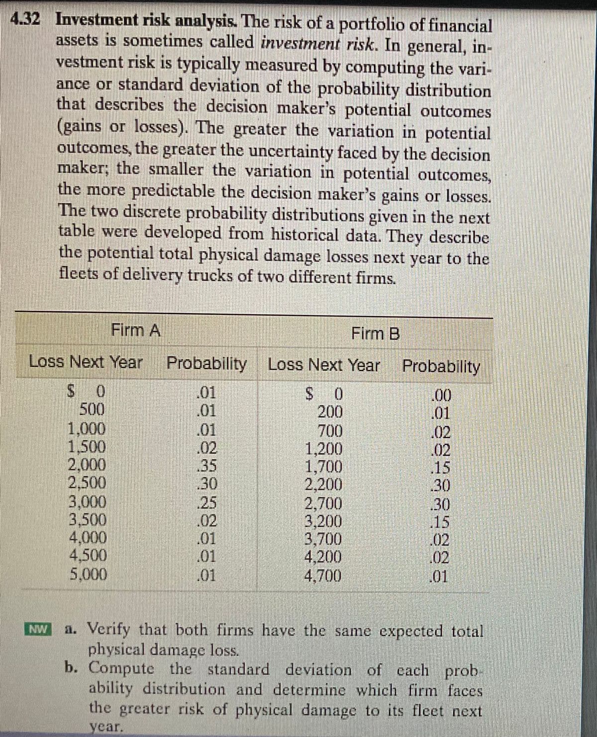
Transcribed Image Text:4.32 Investment risk analysis. The risk of a portfolio of financial
assets is sometimes called investment risk. In general, in-
vestment risk is typically measured by computing the vari-
ance or standard deviation of the probability distribution
that describes the decision maker's potential outcomes
(gains or losses). The greater the variation in potential
outcomes, the greater the uncertainty faced by the decision
maker; the smaller the variation in potential outcomes,
the more predictable the decision maker's gains or losses.
The two discrete probability distributions given in the next
table were developed from historical data. They describe
the potential total physical damage losses next year to the
fleets of delivery trucks of two different firms.
Loss Next Year
SO
500
NW
1,000
1,500
2,000
2.500
Firm A
3.000
3,500
4,000
4,500
5,000
Firm B
Probability Loss Next Year
01
SO 0
.01
200
.01
700
1,200
1,700
2,200
2,700
3.200
3.700
4,200
4,700
30
.01
01
Probability
85984579985
.30
a. Verify that both firms have the same expected total
physical damage loss.
b.
Compute the standard deviation of cach prob.
ability distribution and determine which firm faces
the greater risk of physical damage to its fleet next
year.
Expert Solution
This question has been solved!
Explore an expertly crafted, step-by-step solution for a thorough understanding of key concepts.

This is a popular solution!

Trending now
This is a popular solution!

Step by step
Solved in 3 steps with 8 images

Knowledge Booster


Learn more about
Need a deep-dive on the concept behind this application? Look no further. Learn more about this topic, finance and related others by exploring similar questions and additional content below.Recommended textbooks for you
EBK CONTEMPORARY FINANCIAL MANAGEMENT
Finance
ISBN:
9781337514835
Author:
MOYER
Publisher:
CENGAGE LEARNING - CONSIGNMENT
EBK CONTEMPORARY FINANCIAL MANAGEMENT
Finance
ISBN:
9781337514835
Author:
MOYER
Publisher:
CENGAGE LEARNING - CONSIGNMENT