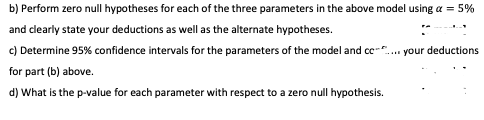
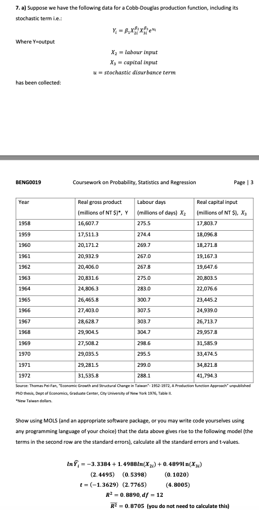
b) Perform zero null hypotheses for each of the three parameters in the above model using a = 5%and clearly state your deductions as well as the alternate hypotheses.c) Determine 95% confidence intervals for the parameters of the model and c-".your deductionsfor part (b) above.d) What is the p-value for each parameter with respect to a zero null hypothesis. 7. a) Suppose we have the following data for a Cobb-Douglas production function, including itsstochastic term i.e.:Y, = B,x: xeWhere Y=outputX2 = labour inputХз — саpital inputu = stochastic disurbance termhas been collected:BENGO019Coursework on Probability, Statistics and RegressionPage | 3YearReal gross productLabour daysReal capital input(millions of NT $)", Y (millions of days) X2(millions of NT $), X3195816,607.7275.517,803.7195917,511.3274.418,096.8196020,171.2269.718,271.8196120,932.9267.019,167.3196220,406.0267.819,647.6196320,831.6275.020,803.5196424,806.3283.022,076.6196526,465.8300.723,445.2196627,403.0307.524,939.0196728,628.7303.726,713.7196829,904.5304.729,957.8196927,508.2298.631,585.9197029,035.5295.533,474.5197129,281.5299.034,821.8197231,535.8288.141,794.3Source: Thomas Pei-Fan, "Economic Growth and Structural Change in Taiwan". 1952-1972, A Production function Approach" unpublishedPhD thesis, Dept of Economics, Graduate Center, City University of New York 1976, Table Il*New Taiwan dollars.Show using MOLS (and an appropriate software package, or you may write code yourselves usingany programming language of your choice) that the data above gives rise to the following model (theterms in the second row are the standard errors), calculate all the standard errors and t-values.InY, = -3.3384 +1.4988ln(X2) + 0.48991 n(X)(2.4495) (0.5398)(0. 1020)t = (-1.3629) (2.7765)R? = 0, 8890, df = 12(4. 8005)R2 = 0.8705 (you do not need to calculate this)

Given: Year Real gross product (millions of NT $)°, Y Labor days (millions of days) X2 Real…

Answered: 7. a) Suppose we have the following…

MATLAB: An Introduction with Applications

6th Edition

ISBN:9781119256830

Author:Amos Gilat

Publisher:Amos Gilat

Chapter1: Starting With Matlab

Section: Chapter Questions

Problem 1P

See similar textbooks

Similar questions

2. Consider a queuing system with a Poisson input and exponential service times. Suppose there is one server and the expected service time is exactly one minute. Compare Ls for the cases where the mean arrival rate is 0.5, 0.9 and 0.99 customers per minute, respectively. Do the same for Lq, Ws, Wq and P(W>5) or the probability of waiting time in the system.
Determine the mean waiting time W for an M/M/2 system when lambda = 2 and μ = 1.2. Compare this with the mean waiting time in an M/M/1 system whose arrival rate is lambda = 1 and service rate is μ = 1.2. Since the arrival rate per server is the same in both cases and service times don’t vary, should the wait times be the same in both cases?
2. A leading researcher in the study of interstate highway accidents proposes that a major cause of many collisions on the interstates is not the speed of the vehicles but rather the difference in speeds of the vehicles. When some vehicles are traveling slowly while other vehicles are traveling at speeds greatly in excess of the speed limit, the faster-moving vehicles may have to change lanes quickly, which can increase the chance of an accident. Thus, when there is a large variation in the speeds of the vehicles in a given location on the interstate, there may be a larger number of accidents than when the traffic is moving at a more uniform speed. The researcher believes that when the standard deviation in speed of vehicles exceeds 10 mph, the rate of accidents is greatly increased. During a 1-hour period of time, a random sample of 50 vehicles is selected from a section of an interstate known to have a high rate of accidents, and their speeds are recorded using a radar gun. The data…
A group of medical professionals is considering theconstruction of a private clinic. If the medical de-mand is high (i.e., there is a favorable market for theclinic), the physicians could realize a net profit of$100,000. If the market is not favorable, they couldlose $40,000. Of course, they don’t have to proceedat all, in which case there is no cost. In the absenceof any market data, the best the physicians can guessis that there is a 50–50 chance the clinic will be suc-cessful. Construct a decision tree to help analyze thisproblem. What should the medical professionals do?
Suppose that a firm can produce a part it uses for $520 per unit, with a fixed cost of $25,000. The company has been offered a contract from a supplier that allows it to purchase the part at a cost of $544 per unit, which includes transportation. The key outputs in the model are the difference in these costs and the decision that results in the lower cost. Assume that the production volume is uncertain. Suppose the manufacturer has enough data and information to estimate that the production volume will be normally distributed with a mean of 1,000 and a standard deviation of 85. Use a 100-trial Monte Carlo simulation to find the average cost difference and percent of trials that result in manufacturing or outsourcing as the best decision. Please include table showing both the cost difference and decision for each trial. Please include the Excel worksheet with all the details with your answer.
1) A cement producer, manufactures and then fills 40kg-bags of powder cement on twodistinct production tracks located in separate suburbs. To determine whether differencesexist between the average fill rates for the two tracks, a random sample of 25 bags fromTrack 1 and a random sample of 16 bags from Track 2 were recently selected. Each bag’sweight was measured and the following information measures from the samples arereported:Production ProductionTrack 1 Track 2n1 = 25 n2 = 16x2 = 40.02 x1 = 39.87 s1 = 0.59 s2 = 0.88 Supervision believes that the fill rates of the two tracks are normally distributed with equalvariances.Construct a 95% confidence interval estimate of the true mean difference between the twotracks.--------------------------------------------------------------------------------------------------------------2) Two independent simple random samples were selected from two normallydistributed populations with unequal variances yielded the following information:Sample 1…
4) Here are data on the lengths of male and female roaches (in mm). Your job is to find out if there is adifference between male and female roaches (this should be two sided - why?).males 15.4 13.9 12.7 9.6 6.6 10.7 9.9 13.3 16.2 9.0 11.4 16.6 12.2females 16.7 16.3 12.8 16.9 15.1 12.8 18.7 18.3 8.6 13.6 15.3 16.2 13.4It's up to you to figure out what the best procedure is, what kind of hypotheses to use, which α to use,what test to use, and so on. Make sure you follow all the appropriate steps. You should probably use Ras you’ll get done much quicker. Remember to very clearly state your results in writing. Never turn in just an R printout .Hint: how do you decide which test to use? What kind of distributions do the data have?
At a toll-booth on-ramp there is a stochastic arrival distribution. Vehicles are counted in 20-second intervals, and vehicle counts are taken in 120 of these time intervals. Based on data collected, no vehicles arrived in 18 of the 120 count intervals. What is the number of the 120 intervals that 3 cars arrived?
Texas Instruments produces computer chips in production runs of 1 million at a time. It has found that the fraction of defective modules can be very different in different production runs. These differences are caused by small variations in the set-up of each production run. Managers have observed that defective rates are roughly triangular, with a lower bound of 0%, and an upper bound of 50%. Defects more likely to be near 10% than any other single value in their range. Now suppose that we have taken a sample of 10 modules, and 2 of them are defective. i. What is the conditional probability of a defective rate less than 25% in this production run?ii. For what number M would you say that the defective rate is equally likely to be above or below M?
A firm is studying the delivery times of two raw material suppliers. The firm is basically satisfied with supplierA and is prepared to stay with that supplier. However, if the firm finds that the mean delivery time of supplierB is less than that of supplier A, it will begin making raw material purchases from supplier B. Assume that 50independent samples from each supplier show the delivery time of supplier A to be 14 days with a standarddeviation of 3 days, while the delivery time of B is shown to be 12.5 days with a standard deviation of 2 days.Testing at a 0.05 level of significance, should the firm switch to supplier B or not? Compute for: null and alternative hypothesis in words level of significance and critical value/s and region (graph it please) compute the test statistic decision state the conclusion
8.7 It is conjectured that when fields are overgrazed by cattle there will be a substantial reduc- tion in the available grass during the subsequent grazing season due to the compaction of the soil. A horticulturist at the state agricultural experiment station designs a study to evaluate the conjec- ture. Twenty-one plots of land of nearly the same soil texture and suitable for grazing are selected for the study. Three grazing regimens selected for evaluation are randomly assigned to 7 plots each. After the 21 plots are subjected to the grazing regimens for four months, the researcher randomly selects 10 soil cores from each plot and measures the bulk density (g/cm3) in each soil core. The mean soil density of the 10 cores from each plot is given in the following table. Grazing Regimen Soil Denisty (g/cm3) Continuous grazing 2.05 3.05 3.12 1.59 3.83 1.53 1.44 Three-week grazing, one-week no grazing 1.20 1.48 3.54 1.03 1.45 1.40 2.68…
(b) A tax consulting firm has 5 counters in its office to receive people who have problemsconcerning their income, wealth and sales taxes. On the average 75 persons arrive in an 8–hour day. Each tax adviser spends 25 minutes on an average on an arrival. If the arrivalsare Poissonly distributed and service times are according to exponential distribution, findiv. Average time a customer spends in the system v. Average waiting time for a customer

SEE MORE QUESTIONS

Recommended textbooks for you

MATLAB: An Introduction with Applications

Statistics

ISBN:

9781119256830

Author:

Amos Gilat

Publisher:

John Wiley & Sons Inc

Probability and Statistics for Engineering and th…

Statistics

ISBN:

9781305251809

Author:

Jay L. Devore

Publisher:

Cengage Learning

Statistics for The Behavioral Sciences (MindTap C…

Statistics

ISBN:

9781305504912

Author:

Frederick J Gravetter, Larry B. Wallnau

Publisher:

Cengage Learning

MATLAB: An Introduction with Applications

Statistics

ISBN:

9781119256830

Author:

Amos Gilat

Publisher:

John Wiley & Sons Inc

Probability and Statistics for Engineering and th…

Statistics

ISBN:

9781305251809

Author:

Jay L. Devore

Publisher:

Cengage Learning

Statistics for The Behavioral Sciences (MindTap C…

Statistics

ISBN:

9781305504912

Author:

Frederick J Gravetter, Larry B. Wallnau

Publisher:

Cengage Learning

Elementary Statistics: Picturing the World (7th E…

Statistics

ISBN:

9780134683416

Author:

Ron Larson, Betsy Farber

Publisher:

PEARSON

The Basic Practice of Statistics

Statistics

ISBN:

9781319042578

Author:

David S. Moore, William I. Notz, Michael A. Fligner

Publisher:

W. H. Freeman

Introduction to the Practice of Statistics

Statistics

ISBN:

9781319013387

Author:

David S. Moore, George P. McCabe, Bruce A. Craig

Publisher:

W. H. Freeman

SEE MORE TEXTBOOKS

7. a) Suppose we have the following data for a Cobb-Douglas production function, including its stochastic term i.e.: Where Ymoutput X2 = labour input X = capital input