America's favorite alcoholic beverage. Are beer, wine, and liquor equally favored by Americans as the alcoholic drink they consume most often? A 2016 Gallup survey interview a random sample of American adults about their alcohol consumption and preferences. Of the 647 non-abstainers who answered the question about which beverage-beer, wine, liquor-they consume most often, 293 selected beer, 218 selected wine, and the remaining 136 selected liquor. Follow the four-step process as illustrated in Example 21.7.
America's favorite alcoholic beverage. Are beer, wine, and liquor equally favored by Americans as the alcoholic drink they consume most often? A 2016 Gallup survey interview a random sample of American adults about their alcohol consumption and preferences. Of the 647 non-abstainers who answered the question about which beverage-beer, wine, liquor-they consume most often, 293 selected beer, 218 selected wine, and the remaining 136 selected liquor. Follow the four-step process as illustrated in Example 21.7.

Holt Mcdougal Larson Pre-algebra: Student Edition 2012
1st Edition
ISBN:9780547587776
Author:HOLT MCDOUGAL
Publisher:HOLT MCDOUGAL
Chapter11: Data Analysis And Probability
Section: Chapter Questions
Problem 8CR

Related questions
Question
21.27 America's favorite alcoholic beverage. Are beer, wine, and liquor equally favored by Americans as the alcoholic drink they consume most often? A 2016 Gallup survey interview a random sample of American adults about their alcohol consumption and preferences. Of the 647 non-abstainers who answered the question about which beverage-beer, wine, liquor-they consume most often, 293 selected beer, 218 selected wine, and the remaining 136 selected liquor. Follow the four-step process as illustrated in Example 21.7.
Transcribed Image Text:Not on the weekend, please
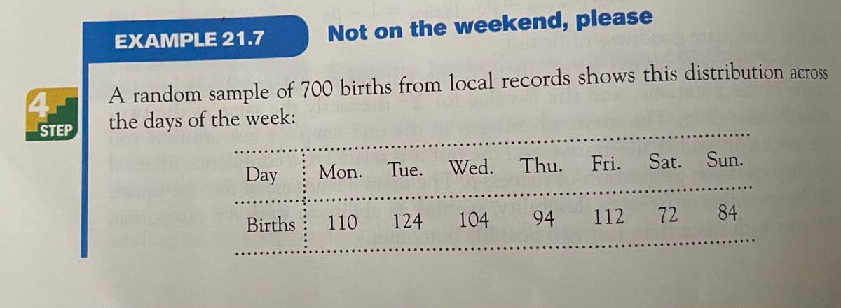
EXAMPLE 21.7
A random sample of 700 births from local records shows this distribution across
the days of the week:
4.
STEP
Day
Mon. Tue. Wed. Thu. Fri. Sat. Sun.
Births
110 124 104 94 112 72 84
..
Transcribed Image Text:Chi-Square Test for in Birth
o test whether some
from the sample data. For each
as the probability of successD
STATE:
any particular day of the week, but modern births
INTERPRETING SIGNIFICANT CHI-SQUARE
may not
ocess step by step.
give
the week?
STATS
IN YOUR
WORLD
on all days of
WEEKEND C
null hypothesis is
ndows down so that they reflect
tal bird strikes. Use software or
You work all w
get 1/7th of all births. So the
rains on the we
Ho: Þ1 = P2=P3 = P4 = P5 = P6 = P7 =
there really be
e in context.
%3D
behind our per
%3D
weather is aga
21.2 investigated a genetic model
P-value of 0.397. Interpret this
heat-resistant phenotypes in F2
%3D
1.
on the East Cc
States, the ans
Going back to
that Sundays
precipitation t
likely explanati
pollution from
cars and truc
for raindrops-
Day
Mon. Tue. Wed. Thu. Fri. Sat. Sun.
Probability
P1 P2 p3 P4 P5 P6 P7
The alternative hypothesis simply says that days are not all equally likely for births
ARE RESULTS
(Ho is not true, not
all p; = ÷):
delay to causE
%3D
epartures from a distribution
y significant, it is important
distribution. Here are three
SOLVE: Check the conditions for inference. We will need to get back to this
weekend.
part later in the chapter.
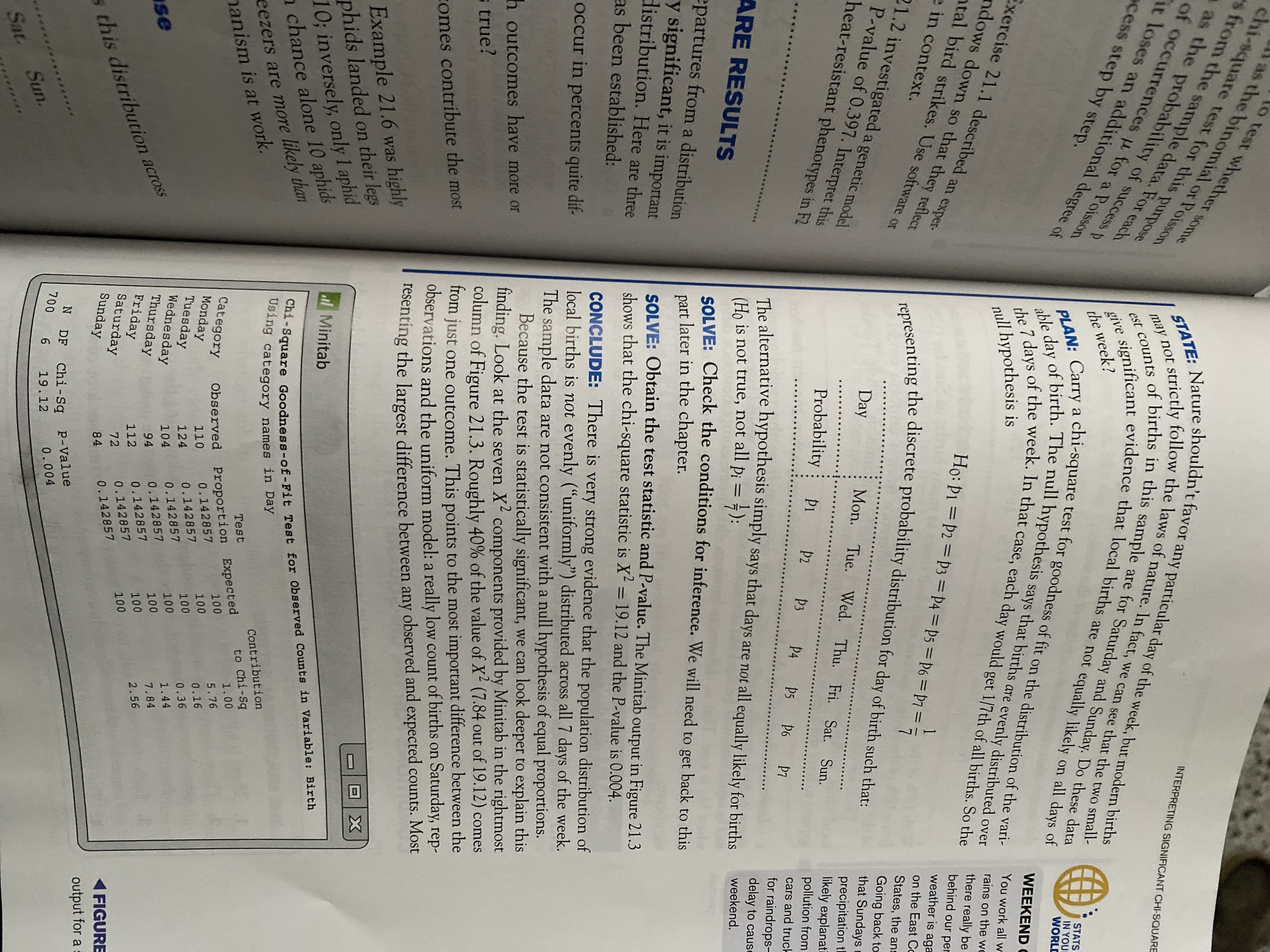
SOLVE: Obtain the test statistic and P-value. The Minitab output in Figure 21.3
shows that the chi-square statistic is X' = 19.12 and the P-value is 0.004.
as been established:
%3D
CONCLUDE: There is very strong evidence that the population distribution of
local births is not evenly (“uniformly") distributed across all 7 days of the week.
The sample data are not consistent with a null hypothesis of equal proportions.
Because the test is statistically significant, we can look deeper to explain this
finding. Look at the seven X components provided by Minitab in the rightmost
column of Figure 21.3. Roughly 40% of the value of X2 (7.84 out of 19.12) comes
occur in percents quite dif-
h outcomes have more or
true?
comes contribute the most
Irom just one outcome. This points to the most important difference between the
observations and the uniform model: a really low count of births on Saturday, rep-
Tesenting the largest difference between any observed and expected counts. Most
Example 21.6 was highly
phids landed on their legs
10; inversely, only 1 aphid
n chance alone 10 aphids
Minitab
eezers are more likely than
nanism is at work.
Contribution
to Chi-Sq
Test
Observed Proportion Expected
0.142857
Category
Monday
Tuesday
Wednesday
Thursday
Friday
100
5.76
110
0.16
124
0.142857
0.36
se
0.142857
104
1.44
across
0.142857
94
7.84
112
0.142857
100
s this distribution
Saturday
2.56
72
0.142857
Sunday
84
0.142857
< FIGURE
output for a :
6 19.12
0.004
Sat. Sun.
Expert Solution
This question has been solved!
Explore an expertly crafted, step-by-step solution for a thorough understanding of key concepts.

This is a popular solution!

Trending now
This is a popular solution!

Step by step
Solved in 2 steps

Recommended textbooks for you
Holt Mcdougal Larson Pre-algebra: Student Edition…
Algebra
ISBN:
9780547587776
Author:
HOLT MCDOUGAL
Publisher:
HOLT MCDOUGAL

College Algebra (MindTap Course List)
Algebra
ISBN:
9781305652231
Author:
R. David Gustafson, Jeff Hughes
Publisher:
Cengage Learning

Glencoe Algebra 1, Student Edition, 9780079039897…
Algebra
ISBN:
9780079039897
Author:
Carter
Publisher:
McGraw Hill
Holt Mcdougal Larson Pre-algebra: Student Edition…
Algebra
ISBN:
9780547587776
Author:
HOLT MCDOUGAL
Publisher:
HOLT MCDOUGAL
College Algebra (MindTap Course List)
Algebra
ISBN:
9781305652231
Author:
R. David Gustafson, Jeff Hughes
Publisher:
Cengage Learning
Glencoe Algebra 1, Student Edition, 9780079039897…
Algebra
ISBN:
9780079039897
Author:
Carter
Publisher:
McGraw Hill