b. Copy and paste that one formula to all the relevant cells in your new sheet. Round your answers to two decimal places. Line Items Year 1 Year 2 Year 3 Year 4 Year 5 Net Sales % % % % Less: Cost of Goods Sold % % % Gross Margin % % % % % Less: Operating Expenses % % % % Less: Taxes % % % % Net Income % % % % %
b. Copy and paste that one formula to all the relevant cells in your new sheet. Round your answers to two decimal places. Line Items Year 1 Year 2 Year 3 Year 4 Year 5 Net Sales % % % % Less: Cost of Goods Sold % % % Gross Margin % % % % % Less: Operating Expenses % % % % Less: Taxes % % % % Net Income % % % % %

Chapter9: Responsibility Accounting And Decentralization
Section: Chapter Questions
Problem 5PB: Financial information for Lighthizer Trading Company for the fiscal year-ended September 30, 20xx,...

Related questions

Question
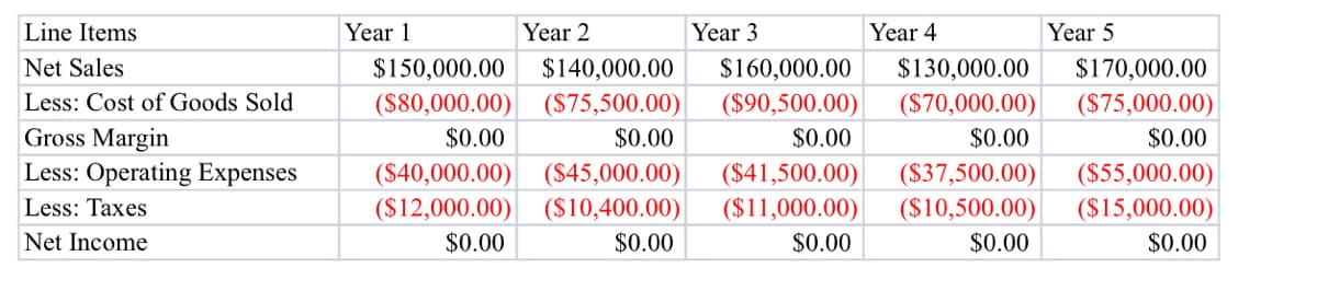
Transcribed Image Text:Line Items
Year 1
Year 2
Year 3
Year 4
Year 5
Net Sales
$150,000.00
$140,000.00
$160,000.00
$130,000.00
$170,000.00
Less: Cost of Goods Sold
($80,000.00)
($75,500.00)
($90,500.00)
($70,000.00)
($75,000.00)
Gross Margin
$0.00
$0.00
$0.00
$0.00
$0.00
Less: Operating Expenses
($40,000.00)
($45,000.00)
($41,500.00)
($11,000.00)
($37,500.00)
($55,000.00)
Less: Taxes
($12,000.00)
($10,400.00)
($10,500.00)
($15,000.00)
Net Income
$0.00
$0.00
$0.00
$0.00
$0.00
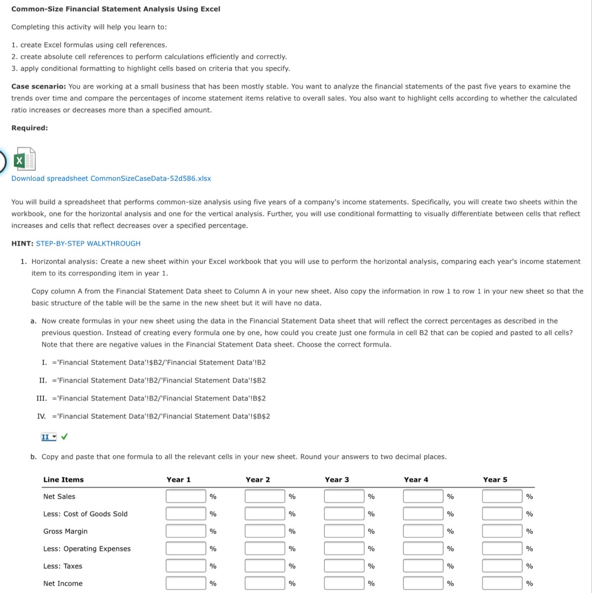
Transcribed Image Text:Common-Size Financial Statement Analysis Using Excel
Completing this activity will help you learn to:
1. create Excel formulas using cell references.
2. create absolute cell references to perform calculations efficiently and correctly.
3. apply conditional formatting to highlight cells based on criteria that you specify.
Case scenario: You are working at a small business that has been mostly stable. You want to analyze the financial statements of the past five years to examine the
trends over time and compare the percentages of income statement items relative to overall sales. You also want to highlight cells according to whether the calculated
ratio increases or decreases more than a specified amount.
Required:
Download spreadsheet CommonSizeCaseData-52d586.xlsx
You will build a spreadsheet that performs common-size analysis using five years of a company's income statements. Specifically, you will create two sheets within the
workbook, one for the horizontal analysis and one for the vertical analysis. Further, you will use conditional formatting to visually differentiate between cells that reflect
increases and cells that reflect decreases over a specified percentage.
HINT: STEP-BY-STEP WALKTHROUGH
1. Horizontal analysis: Create a new sheet within your Excel workbook that you will use to perform the horizontal analysis, comparing each year's income statement
item to its corresponding item in year 1.
Copy column A from the Financial Statement Data sheet to Column A in your new sheet. Also copy the information in row 1 to row 1 in your new sheet so that the
basic structure of the table will be the same in the new sheet but it will have no data.
a. Now create formulas in your new sheet using the data in the Financial Statement Data sheet that will reflect the correct percentages as described in the
previous question. Instead of creating every formula one by one, how could you create just one formula in cell B2 that can be copied and pasted to all cells?
Note that there are negative values in the Financial Statement Data sheet. Choose the correct formula.
I. ='Financial Statement Data'!$B2/'Financial Statement Data'!B2
II. ='Financial Statement Data'!B2/'Financial Statement Data'!$B2
III. ='Financial Statement Data'!B2/'Financial Statement Data'!B$2
IV. ='Financial Statement Data'!B2/'Financial Statement Data'!$B$2
II - V
b. Copy and paste that one formula to all the relevant cells in your new sheet. Round your answers to two decimal places.
Line Items
Year 1
Year 2
Year 3
Year 4
Year 5
Net Sales
%
%
%
%
%
Less: Cost of Goods Sold
%
%
%
%
%
Gross Margin
%
%
%
%
Less: Operating Expenses
%
%
%
%
%
Less: Taxes
%
%
%
%
Net Income
%
%
%
Expert Solution
This question has been solved!
Explore an expertly crafted, step-by-step solution for a thorough understanding of key concepts.

Step by step
Solved in 2 steps with 1 images

Knowledge Booster


Learn more about
Need a deep-dive on the concept behind this application? Look no further. Learn more about this topic, accounting and related others by exploring similar questions and additional content below.Recommended textbooks for you
Principles of Accounting Volume 2
Accounting
ISBN:
9781947172609
Author:
OpenStax
Publisher:
OpenStax College
Financial Accounting: The Impact on Decision Make…
Accounting
ISBN:
9781305654174
Author:
Gary A. Porter, Curtis L. Norton
Publisher:
Cengage Learning

Fundamentals of Financial Management, Concise Edi…
Finance
ISBN:
9781305635937
Author:
Eugene F. Brigham, Joel F. Houston
Publisher:
Cengage Learning
Principles of Accounting Volume 2
Accounting
ISBN:
9781947172609
Author:
OpenStax
Publisher:
OpenStax College
Financial Accounting: The Impact on Decision Make…
Accounting
ISBN:
9781305654174
Author:
Gary A. Porter, Curtis L. Norton
Publisher:
Cengage Learning
Fundamentals of Financial Management, Concise Edi…
Finance
ISBN:
9781305635937
Author:
Eugene F. Brigham, Joel F. Houston
Publisher:
Cengage Learning