Based on what you learned about confidence interval, select ALL the correct statements about the confidence interval. ____Longer interval is more precise __X__A point estimate gives more information than an interval estimate. _____The margin of error is the smallest possible difference between sample mean and population mean. __X___When everything else is same, increasing sample size reduces (lowers) the length of interval. ___X__When everything else is same, increasing confidence level decreases (lowers) the length of interval. ______A point estimate is the single best guess for the parameter while an interval estimate is a range of plausible values for the parameter.


Part 1: One Sample t-Confidence Interval
Based on what you learned about confidence interval, select ALL the correct statements about the confidence interval.
____Longer interval is more precise
__X__A point estimate gives more information than an
_____The margin of error is the smallest possible difference between sample mean and population mean.
__X___When everything else is same, increasing sample size reduces (lowers) the length of interval.
___X__When everything else is same, increasing confidence level decreases (lowers) the length of interval.
______A point estimate is the single best guess for the parameter while an interval estimate is a
______None of these.
The following data represent the Sales (in $1000) data gathered from a marketing efficacy study in Week 1 of December 2019 at a fast-food chain.
Each row is an individual store that was randomly selected for this study.
| Sales(In_Thousands) |
|---|
| 71.63 |
| 62.37 |
| 63.2 |
| 74.48 |
| 36.83 |
| 70.35 |
| 43.48 |
| 43.57 |
| 47.5 |
| 49.63 |
| 49.78 |
| 51.59 |
| 58.22 |
| 60.14 |
| 61.58 |
| 67.23 |
| 70.06 |
| 75.92 |
| 77.4 |
| 85.46 |
| 87.55 |
| 89.23 |
| 60.95 |
| 71.58 |
| 64.92 |
a. Use Excel to create a
Using the result, fill in the blanks of the following statements rounded properly to 2 decimal places.
The average (in $1000) sales is______________.
The margin of error (in $1000) for 98% confidence interval is_____________.
The lower limit (in $1000) of 98% confidence interval for average sales is____________.
The upper limit (in $1000) of 98% confidence interval for average sales is_____________.
Based on your lower and upper limits of a 98% confidence interval for average sales, is it plausible that the average sales (in $1000) for all such stores be 65 in Week 1 of December? Yes or No
because
_____65 is between lower and upper values.
_____65 is NOT between lower and upper values.
______65 is a value in the given data.
______65 is NOT a value in the given data.
__X____None of these.
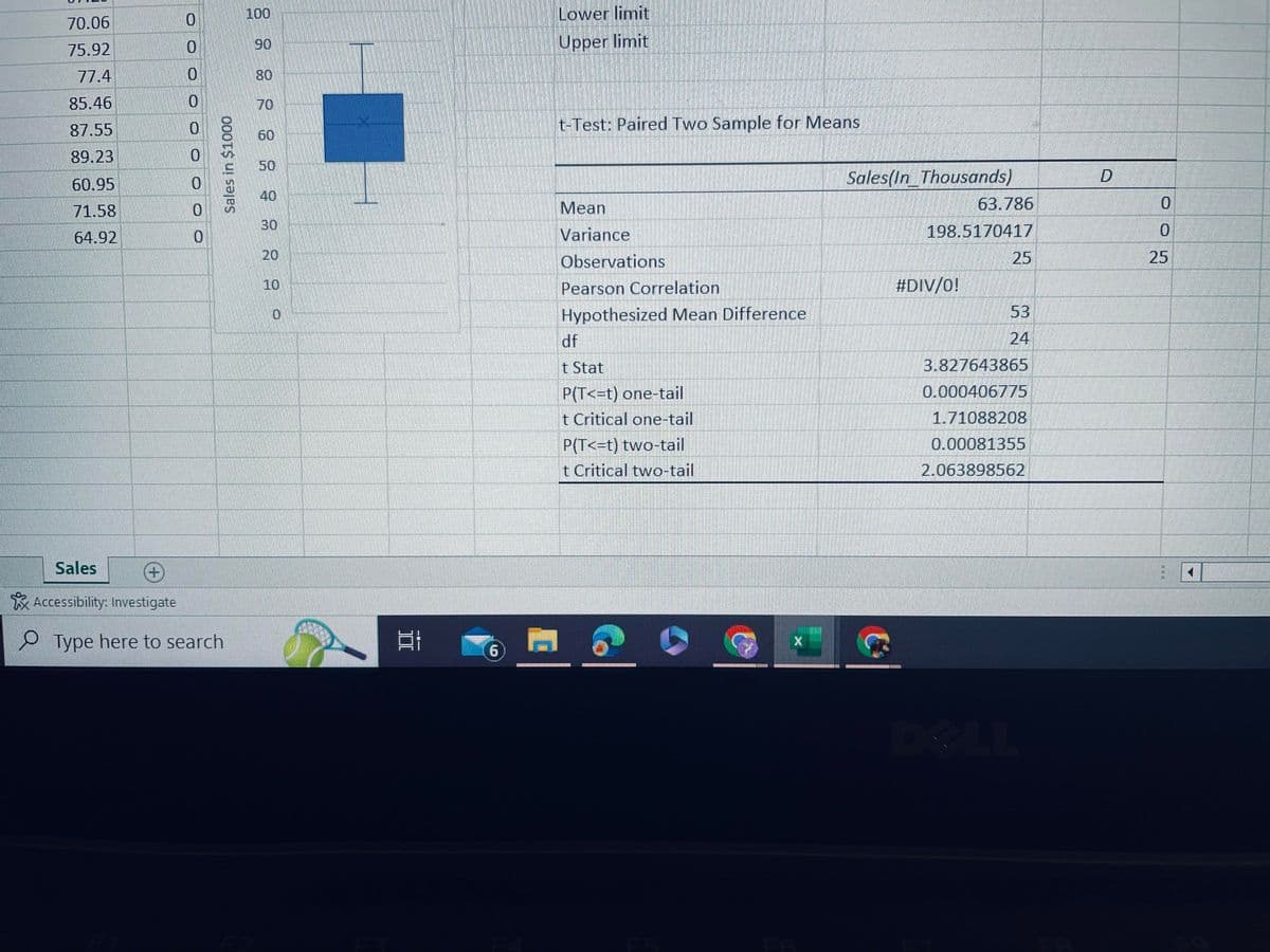
Part 2: One Sample t-Test
a. Use Excel to perform a one-sample t test to test the claim that the average sales (in $1000) for all such stores is different from 65 in Week 1 of December.
The p-value for this test is (rounded to 4 decimal places)_______________
At 0.02 significance level, the correct conclusion for this test is
_____There is enough evidence that the average sales (in $1000) for all such stores is different from 65 in Week 1 of December
____There is NO enough evidence that the average sales (in $1000) for all such stores is different from 65 in Week 1 of December
__X__None of these.
b. Select ONLY the necessary requirements (or assumptions) met in this analysis to confirm that our results from the one-sample t procedures are valid. Make sure to use Excel to create a histogram and boxplot for the data.
__x___There is a random sample of data.
_____There is NO random sample of data.
___x__The sample is large enough.
_____It is given that the population has a
__x___The histogram and boxplot shows it is safe to assume sample is selected from a population with a Normal distribution.
___x___The boxplot shows the sample has no outliers.
______None of these.
c. Do your conclusions based on confidence interval and p-value indicate the same thing?
____Yes, because we use matching confidence level and significance level.
__x__No, they don't have to be same.
![1
2
3
4
5
6
7
8
9
10
12
13
A
Sales(In_Thousands) D
16
17
18
19
20
21
22
23
24
25
26
27
28
29
Ready
71.63
62.37
63.2
74.48
36.83
70.35
43.48
43.57
47.5
49.63
49.78
51.59
58.22
60.14
61.58
67.23
70.06
75.92
77.4
85.46
87.55
89.23
60.95
71.58
64.92
B
Sales
+
Accessibility: Investigate
0
0
0
0
0
10
0
0
0
0
0
10
0
0
0
10
0
0
0
0
0
0
0
0
0
Type here to search
C
Frequency
Sales in $1000
01 00 1 10 in
5
OPNWA
0
100
90
80
70
60
50
40
30
10
[36.83, 47.31]
D
Histogram
(47.31, 57.79)
E
Boxplot
(57.79,68.27)
Sales in $1000
100
(68.27,78.75)
6
F
(EZ 68 52 84)
Mean
Standard Error
Median
Mode
Standard Deviation
Sample Variance
Kurtosis
Skewness
Range
Minimum
Maximum
G
Lower limit
Upper limit
Sales(In_Thousands)
Sum
Count
Confidence Level(98.0%)
t-Test: Paired Two Sample for Means
Mean
Variance
Observations
Pearson Correlation
Hypothesized Mean Difference
H
63.786
2.817921515
#N/A
63.2
14.08960758
198.5170417
-0.595149066
-0.01719769
52.4
36.83
89.23
1594.65
Sales(In Thousands)
#DIV/0!
25
7.022709799 Margin of error
63.786
198.5170417
25
53
I
D
0
0
25
E
+](/v2/_next/image?url=https%3A%2F%2Fcontent.bartleby.com%2Fqna-images%2Fquestion%2F1402ae89-ddd6-4d3d-be54-d5c5eea3ccbf%2F6b26a23c-d1e8-4feb-867e-84d448375b95%2Fa389q5_processed.jpeg&w=3840&q=75)


Trending now
This is a popular solution!

Step by step
Solved in 3 steps

