Below is a data for rainfall and runoff volume in Marfa Texas Rainfall 12 14 17 23 30 40 47 Run off 4 10 13 15 15 25 27 26 Rain fall 55 67 72 81 96 112 127 Run off 38 46 53 70 82 99 100 a. Build a linear regression model. b. Find the residual of all the data points. What is the average value of these residuals? What is the average value of the residuals squared? c. What is the total variance of the runoff volume? What proportion of the observed variation of runoff volume can be attributed to the linear relationship between rainfall and run off?
Q: The following data were collected during a study of consumer buying patterns: Observation y 1 15 74…
A: (1) Use EXCEL to construct the scatter plot. EXCEL procedure: Go to EXCEL Go to Insert menu…
Q: The following data give the experience (in years) and monthly salaries (in hundreds of pesos) of…
A: Regression Equation: When we want to predict the value of one variable, say Y, from the given value…
Q: A population of grades for a statistics class of six students is given below: 80 74 65 84 85 70…
A: From the provided information, The population data is as follow: 80, 74, 65, 84, 85, 70
Q: The results of a multiple regression analysis, using Minitab, follow. Analysis of Variance Source…
A: Hey, since there are multiple subparts posted, we will answer first three subparts. If you want any…
Q: Listed below are paired data consisting of movie budget amounts and the amounts that the movies…
A:
Q: For the following data set, how much of the variation in the outcome variable is explained by the…
A: The table shows x and y values.
Q: The table below lists heights and weights of 10 female and 10 male professional basketball players:…
A: Regression equation is given by, Correlation coefficient is given by,
Q: A sales manager collected the following data on annual sales for new customer accounts and the…
A: Given data, Year of experience Annual sales 1 80 2 89 3 94 3 90 5 104 6 101 7 110…
Q: The final test and exam averages for 20 randomly selected students taking a course in engineering…
A: Since you have posted a question with multiple sub-parts, we will solve first three sub- parts for…
Q: 2. Given the following datalist of the height and weight pairs: Height 68 69 70 70 71 71 72 72 73 73…
A: Correlation coefficient There is strong positive linear relationship between the height and…
Q: For a sample of 8 employees, a personnel director has collected the following data on ownership of…
A: As per our guidelines we can solve first three subpart and rest can be reposted. Solution-: X=Years…
Q: The following table shows economic development measured in per capita income PCINC. Year PCINC Year…
A: Hey, since there are multiple subparts posted, we will answer first three subparts. If you want any…
Q: Consider the following annual sales data for 2001-2008: Year Sales 2001 2…
A: The given data is Year Sale 2001 2 2002 4 2003 10 2004 8 2005 14 2006 18 2007 17…
Q: a) Is the relationship between Age and Earn statistically significant? b) The variance of the…
A: Given , value of R2 = 0.05 , then correlation coefficient = R = 0.05 = 0.2236 a) Is the…
Q: The following table presents data from a solar energy project: X (Deflexión) Y (Flujo de Calor)…
A: Hello thanks for your question. Since you have posted a question with multiple sub-parts, I will…
Q: Subject Weight [Ib] Hg] 1 165 130 2 167 133 3 180 150 4 155 128 5 212 151 6 175 146 7 190 150 8 210…
A:
Q: A study was conducted to determine whether the final grade of a student in an introductory…
A: Since you have posted multiple sub-parts, we will solve the first three sub-parts for you. To get…
Q: For the following data, if a correlation coefficient of r = 0.9679 is calculated, how much of the…
A: We know that the percentage of variation is the dependent variable that can be explained by an…
Q: The following are the number of grams of water and the number of grams of carbohydrates for a random…
A: X:- 83.93, 80.76, 87.66, 85.20, 72.85, 84.61, 83.61 Y:- 15.25, 16.55, 11.10, 13.01, 24.27, 14.13,…
Q: Listed below are paired data consisting of movie budget amounts and the amounts that the movies…
A:
Q: The following table shows the annual family income of the students enrolled in the JRMSU-TC and…
A: Solution-: Let, X=Annual family income (Pesos) (in '000) and Y=General weighted average (%) We have…
Q: Sales Representative Actual Sales, Y 30 60 40 60 30 40 40 50 30 70 ABCDEFGH с D I J Estimated Sales,…
A: Given : Sales Representative Actual Sales , Y Estimated Sales, Y' A 30 42.6316 B 60 66.3156…
Q: The following table shows data for the cost of natural gas in Maryland (in dollars per Million Btu)…
A: a). Here, the price can be predicted using the year. Therefore, the price is the response variable…
Q: Listed below are paired data consisting of movie budget amounts and the amounts that the movies…
A: Introduction: Consider that x is the independent variable and y is the dependent variable. The size…
Q: 13. What proportion of the variance in Course % is attributable to the regression model? A- .568…
A: 13) The proportion of variance in course is attributable to the regression model is R-square.
Q: A researcher wants to determine if the number of years of education for a parent correlates with the…
A:
Q: The following table compares the completion percentage and interception percentage of 55 NFL…
A: Given: x y 55 4.7 58 4.3 58 3.8 60 3.7 64 2.8
Q: Below is a data for rainfall and runoff volume in Marfa Texas Rainfall 5 12 14 17 23 30 40 47 Run…
A: Given that Following table shows the calculations: X Y X^2 Y^2 XY 5 4 25 16 20 12 10…
Q: 6. The following chart shows the winning Olympic Men's High Jump distances. Year Height (inches)…
A: (a) Use EXCEL to construct the scatter plot. EXCEL procedure: Go to EXCEL Go to Insert menu…
Q: Suppose a doctor measures the height, x, and head circumference, y, of 11 children and obtains the…
A: The correlation coefficient (r)=0.904 we know that, coefficient of determination measure…
Q: You were given a dataset that includes 100 datapoints for expenses in Canadian dollars and waste in…
A: The independent variable is Expenses. The dependent variable is Waste amount. This is simple linear…
Q: The following correlations were computed as part of a multiple regression analysis that used…
A: Multiple Regression genreal form Y=βo+β1X1+β2X2+...+βnXn+e Where Y=dependent variables X1, X2,…
Q: A sample has 11 paired observations, Use the xas the independent variable and the y as the dependent…
A:
Q: The Kak Ramah company supplies vegetables to shop as wholesales. The demand for the vegetables…
A: The data given is: Price per kg (RM) Demand (kg) 20 700 22 685 24 630 26 580 28 515…
Q: Run a regression analysis on the following bivariate set of data with y as the response variable. y…
A:
Q: is there relationship between the life expectancy for men and the life expectancy for women in a…
A: Given data represents a random sample of non -industrialized countries was selected and the life…
Q: The Following data is given for the period 1999-2003 Interest rate Inflation…
A: Taking interest rate as independent variable (X) and inflation rate as dependent variable (Y).
Q: Listed Below are amounts of bills for dinner and the amounts of tips thet were left. is there…
A: Note: Thank you for the question. Since multiple subparts are posted, according to our policy, we…
Q: Based on the data shown below, calculate the regression line. y 5.55 6 6.92 7 7.29 8 9.96 9 10.33 10…
A: Regression Equation: When we want to predict the value of one variable, say Y, from the given value…
Q: The following are the number of grams of water and the number of grams of carbohydrates for a random…
A: Since you have asked multiple subparts, we will solve first three subparts for you. To get remaining…
Q: A highway employee performed a regression analysis of the relationship between the number of…
A: The answer can be given by given Data and formulas for s and R.
Q: For the data given below, fill in the blanks, using Formulas, Descriptive Statistics and Regression…
A: Hello. Since your question has multiple sub-parts, we will solve first three sub-parts for you. If…
Q: Listed below are paired data consisting of movie budget amounts and the amounts that the movies…
A: Step-by-step procedure to find the regression equation using Excel: In Excel sheet, enter Budget in…
Q: The personnel director of a large hospital is interested in determining the relationship (if any)…
A: Solution
Q: The following table gives information on the limited tread warranties (in thousands of miles) and…
A: "Since you have posted a question with multiple subparts, we will solve first 3 sub-parts for you.…
Q: The following data represent the time between eruptions and the length of eruption for 9 randomly…
A: Solution: From the given information, the coefficient of determination is 85.7%.
Q: 4. The population in the city of Houston from 1900 to 2010 is given below: Year Population 44,633…
A: a. Consider x (year) be the independent variable and y (population) be the dependent variable. Excel…
Q: The following data were used in a regression study. TL TI Observation Observation 1 4 5 6. 5 7 4. 3…
A: Given: n = 9 Formula Used: The equation of regression is: y^ = a + bX Where, a is intercept b is…
Q: Listed below are paired data consisting of movie budget amounts and the amounts that the movies…
A: Given, Predictor variable X=Budget ($)in Millions Predicted variable Y=Gross($)in Millions n=15 The…
Q: The following are sample data provided by a movingcompany on the weights of six shipments, the…
A: (a) Excel Procedure: Enter the data for y, x1 and x2 in Excel>Data> Data Analysis.>…
Please provide solution and logic for questions attached, thanks!
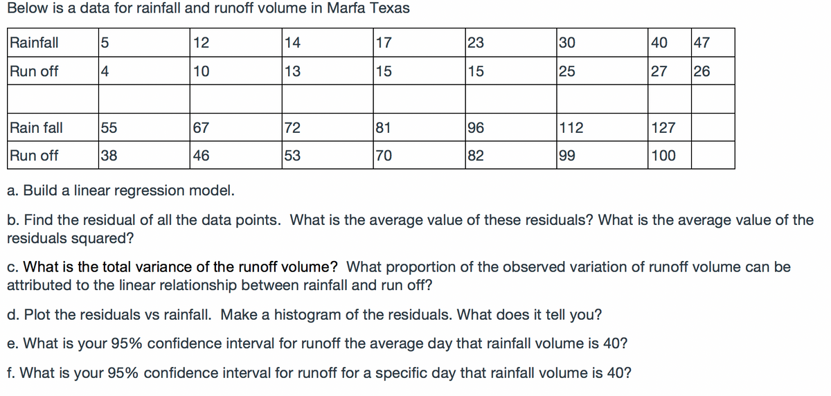
Step by step
Solved in 4 steps
- The following data is a regression model where the U.S. Department of Transportation has tried to relate the rate of fatal traffic accidents (per 1000 licenses) to the percentage of motorists under the age of 21. Data has been collected for 42 major cities in the United States. SUMMARY OUTPUT Regression Statistics Multiple R 0.83938748 R Square 0.70457134 Adjusted R Square 0.69718562 Standard Error 0.58935028 Observations 42 ANOVA df SS MS F Regression 1 33.13441764 33.1344 95.3964 Residual 40 13.89335048 0.34733 Total 41 47.02776812 Coefficients Standard Error t Stat P-value Intercept -1.5974138 0.371671454 -4.2979 0.00010 Percent Under 21 0.28705317 0.029389769 9.76711 3.79E-9…Consider the following computer output from a multiple regression analysis relating the price of a used car to the variables: age of car, mileage, and safety rating. Coefficients Coefficients Standard Error t� Stat P-value Intercept 42465.6942465.69 5320.545320.54 7.9817.981 0.00000.0000 Age (Year) −21096.02−21096.02 2551.522551.52 −8.268−8.268 0.00000.0000 Mileage(in Thousands) −1312.73−1312.73 103.02103.02 −12.743−12.743 0.00000.0000 Safety Rating 1533.821533.82 165.72165.72 9.2559.255 0.00000.0000 Does the sign of the coefficient for the variable safety rating make sense?A researcher notes that, in a certain region, a disproportionate number of software millionaires were born around the year 1955. Is this a coincidence, or does birth year matter when gauging whether a software founder will besuccessful? The researcher investigated this question by analyzing the data shown in the accompanying table. Complete parts a through c below. a. Find the coefficient of determination for the simple linear regression model relating number (y) of software millionaire birthdays in a decade to total number (x) of births in the region. Interpret the result. The coefficient of determination is 1.___? (Round to three decimal places as needed.) This value indicates that 2.____ of the sample variation in the number of software millionaire birthdays is explained by the linear relationship with the total number of births in the region. (Round to one decimal place as needed.) b. Find the coefficient of determination for the simple linear regression model…
- A sales manager collected the following data on annual sales for new customer accounts and the number of years of experience for a sample of 10 salespersons. Salesperson Years of Experience Annual Sales ($1000s) 1 1 80 2 3 97 3 4 92 4 4 102 5 6 103 6 8 111 7 10 119 8 10 123 9 11 117 10 13 136 Develop a scatter diagram for these data with years of experience as the independent variable. Develop an estimated regression equation that can be used to predict annual sales given the years of experience. Use the estimated regression equation to predict annual sales for a salesperson with 9 years of experience.A part of the output of a regression analysis of Y against X using Excel is given below:SUMMARY OUTPUTRegression StatisticsMultiple R 0.954704R Square 0.91146Adjusted R Square 0.896703Standard Error 28.98954Observations 8ANOVAdf SS MS F Significance FRegression 1 51907.64 51907.64Residual 6 5042.361 840.3936Total 7 56950Coefficients Standard Error t Stat P-valueIntercept 45.2159 39.8049Age 5.3265 0.6777a. State the estimated regression line and interpret the slope coefficient.Consider the following computer output from a multiple regression analysis relating the price of a used car to the variables: age of car, mileage, and safety rating. Coefficients Coefficients Standard Error t� Stat P-value Intercept 38356.1138356.11 4686.294686.29 8.1858.185 0.00000.0000 Age (Year) −18219.29−18219.29 2196.312196.31 −8.295−8.295 0.00000.0000 Mileage(in Thousands) 1149.561149.56 1897.651897.65 0.6060.606 0.54720.5472 Safety Rating 1396.751396.75 159.64159.64 8.7498.749 0.00000.0000 Does the sign of the coefficient for the variable mileage make sense?
- The Following data is given for the period 1999-2003 Interest rate Inflation i π 1999 4.7 4.4 2000 4.6 5.4 2001 6.3 5.7 2002 4.8 4.6 2003 2.9 2.4 Obtain residuals of the regression. Calculate variance of the residuals and the standard errors of the parametersConsider the following computer output of a multiple regression analysis relating annual salary to years of education and years of work experience. Regression Statistics Multiple R 0.73520.7352 R Square 0.54050.5405 Adjusted R Square 0.52050.5205 Standard Error 2131.18202131.1820 Observations 4949 ANOVA dfdf SSSS MSMS F� Significance F� Regression 22 245,793,126.4218245,793,126.4218 122,896,563.2109122,896,563.2109 27.058227.0582 1.7E-081.7E-08 Residual 4646 208,929,085.5374208,929,085.5374 4,541,936.64214,541,936.6421 Total 4848 454,722,211.9592454,722,211.9592 Coefficients Standard Error t� Stat P-value Lower 95%95% Upper 95%95% Intercept 14268.6823614268.68236 2,521.08442,521.0844 5.65975.6597 0.0000009340.000000934 9194.00279194.0027 19,343.362119,343.3621 Education (Years) 2352.26982352.2698 337.1115337.1115 6.97776.9777 0.000000010.00000001 1673.69951673.6995 3030.84013030.8401 Experience (Years) 832.2096832.2096…The following data on exposure to alpha particles on cell abnormalities. Exposure abnormalities 0.106 2 0.193 5 0.511 13 0.527 15 1.08 25 1.62 28 1.73 36 2.36 45 2.72 56 3.12 59 3.88 63 4.18 60 Construct the scatter plot and compute the regression line Compute the residuals and graph the residual plot Comment on any features you see in these data.
- The following data shows the percent of females 18 years old or older who were overweight in the number of years indicated, judging on the basis of BMI. Year, Percent Obese 3 , 23.3 4, 23.7 5, 24.3 6, 25.6 7, 25.2 8, 27.6 9, 26.8 Using regression equation, predict the percent of overweight females in year 15.Consider the following computer output of a multiple regression analysis relating annual salary to years of education and years of work experience. Regression Statistics Multiple R 0.73720.7372 R Square 0.54340.5434 Adjusted R Square 0.52350.5235 Standard Error 2120.66062120.6606 Observations 4949 ANOVA dfdf SSSS MSMS F� Significance F� Regression 22 246,191,336.3605246,191,336.3605 123,095,668.1803123,095,668.1803 27.371627.3716 1.5E-081.5E-08 Residual 4646 206,871,255.7619206,871,255.7619 4,497,201.21224,497,201.2122 Total 4848 453,062,592.1224453,062,592.1224 Coefficients Standard Error t� Stat P-value Lower 95%95% Upper 95%95% Intercept 14262.1701214262.17012 2,508.63812,508.6381 5.68525.6852 0.0000008560.000000856 9212.54359212.5435 19,311.796719,311.7967 Education (Years) 2354.97312354.9731 335.4472335.4472 7.02047.0204 0.0000000080.000000008 1679.75291679.7529 3030.19333030.1933 Experience (Years) 830.0759830.0759…Consider the following computer output of a multiple regression analysis relating annual salary to years of education and years of work experience. Regression Statistics Multiple R 0.73720.7372 R Square 0.54340.5434 Adjusted R Square 0.52350.5235 Standard Error 2120.66062120.6606 Observations 4949 ANOVA dfdf SSSS MSMS F� Significance F� Regression 22 246,191,336.3605246,191,336.3605 123,095,668.1803123,095,668.1803 27.371627.3716 1.5E-081.5E-08 Residual 4646 206,871,255.7619206,871,255.7619 4,497,201.21224,497,201.2122 Total 4848 453,062,592.1224453,062,592.1224 Coefficients Standard Error t� Stat P-value Lower 95%95% Upper 95%95% Intercept 14262.1701214262.17012 2,508.63812,508.6381 5.68525.6852 0.0000008560.000000856 9212.54359212.5435 19,311.796719,311.7967 Education (Years) 2354.97312354.9731 335.4472335.4472 7.02047.0204 0.0000000080.000000008 1679.75291679.7529 3030.19333030.1933 Experience (Years) 830.0759830.0759…