*BOLD MEANS I NEED HELP ON THIS SECTION. PLEASE LOOK AT IMAGES. The Stanford University Heart Transplant Study (1974) was conducted to determine whether an experimental heart transplant program increased lifespan. Each patient entering the program was designated an official heart transplant candidate, meaning that he was gravely ill and would most likely benefit from a new heart. Some patients got a transplant and some did not. Of the 34 patients in the control group, 4 were alive at the end of the study. Of the 69 patients in the treatment group, 24 were alive. The contingency table below summarizes these results. ControlTreatmentTotalAlive42428Dead304575Total3469103a) What proportion of patients in the treatment group were still alive at the end of the study? .348Correct (Round to three decimal places.)b) What proportion of patients in the control group were still alive at the end of the study? .118 (Round to three decimal places.)c) What are the claims being tested?H0H0: The experimental heart transplant program Select an answer increases does not increase Correct lifespan.HAHA: The experimental heart transplant program Select an answer increases does not increase Correct lifespan.d) One approach for investigating whether or not the treatment is effective is to use a randomization technique. The paragraph below describes the set up for such approach, if we were to do it without using statistical software. Fill in the blanks with a number or phrase, whichever is appropriate.We write alive on Correct cards representing patients who were alive at the end of the study, and dead on Correct cards representing patients who were not. Then, we shuffle these cards and split them into two groups: one group of size Correct representing treatment, and another group of size Correct representing control. We calculate the difference between the proportion of "alive" cards in the treatment and control groups (treatment - control) and record this value. We complete this process 100 times to build a distribution centered at _____?Lastly, we calculate the fraction of simulations where the simulated differences in proportions are even more favorable to the alternative hypothesis than________? the difference in proportions from the original sample. If this fraction is low, we conclude that it is unlikely to have observed such an outcome by chance and that the null hypothesis should be rejected in favor of the alternative. e) What is the estimated p-value, based on the simulation results above? (Assume the simulation differences in proportions shown above are subtracted in the same order as your difference in sample proportions.) g) Write an appropriate conclusion about the alternative hypothesis in context. The Stanford University Heart Transplant Study (1974) was conducted to determine whether anexperimental heart transplant program increased lifespan. Each patient entering the program wasdesignated an official heart transplant candidate, meaning that he was gravely ill and would most likelybenefit from a new heart. Some patients got a transplant and some did not. Of the 34 patients in thecontrol group, 4 were alive at the end of the study. Of the 69 patients in the treatment group, 24 werealive. The contingency table below summarizes these results.Control TreatmentTotalAlive42428Dead304575Total3469103a) What proportion of patients in the treatment group were still alive at the end of the study? .348 vo (Round to three decimal places.)b) What proportion of patients in the control group were still alive at the end of the study? .118(Roundto three decimal places.)c) What are the claims being tested?Ho: The experimental heart transplant program does not increase Vo lifespan.HA: The experimental heart transplant program increaseso lifespan.d) One approach for investigating whether or not the treatment is effective is to use a randomizationtechnique. The paragraph below describes the set up for such approach, if we were to do it without usingstatistical software. Fill in the blanks with a number or phrase, whichever is appropriate.We write alive on 28o cards representing patients who were alive at the end of the study, anddead on 75o cards representing patients who were not. Then, we shuffle these cards and splitthem into two groups: one group of size 69V o representing treatment, and another group of size34o representing control. We calculate the difference between the proportion of "alive" cards inthe treatment and control groups (treatment - control) and record this value. We complete this process 100times to build a distribution centered atLastly, we calculate the fraction of simulations where thesimulated differences in proportions are even more favorable to the alternative hypothesis thanthe difference in proportions from the original sample. If this fraction is low, we conclude that it is unlikelyto have observed such an outcome by chance and that the null hypothesis should be rejected in favor ofthe alternative. -0.25-0.15-0.050.050.150.25Simulated differences in proportionse) What is the estimated p-value, based on the simulation results above? (Assume the simulationdifferences in proportions shown above are subtracted in the same order as your difference in sampleproportions.)f) At the 5% level of significance, we should rejecto the null hypothesis.g) Write an appropriate conclusion about the alternative hypothesis in context.Submit Ouoction.......

Name: *BOLD MEANS I NEED HELP ON THIS SECTION. PLEASE LOOK AT IMAGES. The St
Uploaded: 2024-03-20T07:06:27.000Z
Channel: Bartleby
Description: *BOLD MEANS I NEED HELP ON THIS SECTION. PLEASE LOOK AT IMAGES. The Stanford University Heart Transplant Study (1974) was conducted to determine whether an experimental heart transplant program increased lifespan. Each patient entering the program wa

The 2x2 contingency table is given We can calculate the sample proportions of the 2 groups.

Math

Statistics

*BOLD MEANS I NEED HELP ON THIS SECTION. PLEASE LOOK AT IMAGES. The Stanford University Heart Transplant Study (1974) was conducted to determine whether an experimental heart transplant program increased lifespan. Each patient entering the program was designated an official heart transplant candidate, meaning that he was gravely ill and would most likely benefit from a new heart. Some patients got a transplant and some did not. Of the 34 patients in the control group, 4 were alive at the end of the study. Of the 69 patients in the treatment group, 24 were alive. The contingency table below summarizes these results. Control Treatment Total Alive 4 24 28 Dead 30 45 75 Total 34 69 103 a) What proportion of patients in the treatment group were still alive at the end of the study? .348Correct (Round to three decimal places.) b) What proportion of patients in the control group were still alive at the end of the study? .118 (Round to three decimal places.) c) What are the claims being tested? H0H0: The experimental heart transplant program Select an answer increases does not increase Correct lifespan. HAHA: The experimental heart transplant program Select an answer increases does not increase Correct lifespan. d) One approach for investigating whether or not the treatment is effective is to use a randomization technique. The paragraph below describes the set up for such approach, if we were to do it without using statistical software. Fill in the blanks with a number or phrase, whichever is appropriate. We write alive on Correct cards representing patients who were alive at the end of the study, and dead on Correct cards representing patients who were not. Then, we shuffle these cards and split them into two groups: one group of size Correct representing treatment, and another group of size Correct representing control. We calculate the difference between the proportion of "alive" cards in the treatment and control groups (treatment - control) and record this value. We complete this process 100 times to build a distribution centered at _____?Lastly, we calculate the fraction of simulations where the simulated differences in proportions are even more favorable to the alternative hypothesis than________? the difference in proportions from the original sample. If this fraction is low, we conclude that it is unlikely to have observed such an outcome by chance and that the null hypothesis should be rejected in favor of the alternative. e) What is the estimated p-value, based on the simulation results above? (Assume the simulation differences in proportions shown above are subtracted in the same order as your difference in sample proportions.) g) Write an appropriate conclusion about the alternative hypothesis in context.

*BOLD MEANS I NEED HELP ON THIS SECTION. PLEASE LOOK AT IMAGES. The Stanford University Heart Transplant Study (1974) was conducted to determine whether an experimental heart transplant program increased lifespan. Each patient entering the program was designated an official heart transplant candidate, meaning that he was gravely ill and would most likely benefit from a new heart. Some patients got a transplant and some did not. Of the 34 patients in the control group, 4 were alive at the end of the study. Of the 69 patients in the treatment group, 24 were alive. The contingency table below summarizes these results. Control Treatment Total Alive 4 24 28 Dead 30 45 75 Total 34 69 103 a) What proportion of patients in the treatment group were still alive at the end of the study? .348Correct (Round to three decimal places.) b) What proportion of patients in the control group were still alive at the end of the study? .118 (Round to three decimal places.) c) What are the claims being tested? H0H0: The experimental heart transplant program Select an answer increases does not increase Correct lifespan. HAHA: The experimental heart transplant program Select an answer increases does not increase Correct lifespan. d) One approach for investigating whether or not the treatment is effective is to use a randomization technique. The paragraph below describes the set up for such approach, if we were to do it without using statistical software. Fill in the blanks with a number or phrase, whichever is appropriate. We write alive on Correct cards representing patients who were alive at the end of the study, and dead on Correct cards representing patients who were not. Then, we shuffle these cards and split them into two groups: one group of size Correct representing treatment, and another group of size Correct representing control. We calculate the difference between the proportion of "alive" cards in the treatment and control groups (treatment - control) and record this value. We complete this process 100 times to build a distribution centered at _?Lastly, we calculate the fraction of simulations where the simulated differences in proportions are even more favorable to the alternative hypothesis than____? the difference in proportions from the original sample. If this fraction is low, we conclude that it is unlikely to have observed such an outcome by chance and that the null hypothesis should be rejected in favor of the alternative. e) What is the estimated p-value, based on the simulation results above? (Assume the simulation differences in proportions shown above are subtracted in the same order as your difference in sample proportions.) g) Write an appropriate conclusion about the alternative hypothesis in context.

MATLAB: An Introduction with Applications

6th Edition

ISBN:9781119256830

Author:Amos Gilat

Publisher:Amos Gilat

Chapter1: Starting With Matlab

Section: Chapter Questions

Problem 1P

See similar textbooks

Related questions

Concept explainers

Topic Video

Question

*BOLD MEANS I NEED HELP ON THIS SECTION. PLEASE LOOK AT IMAGES.

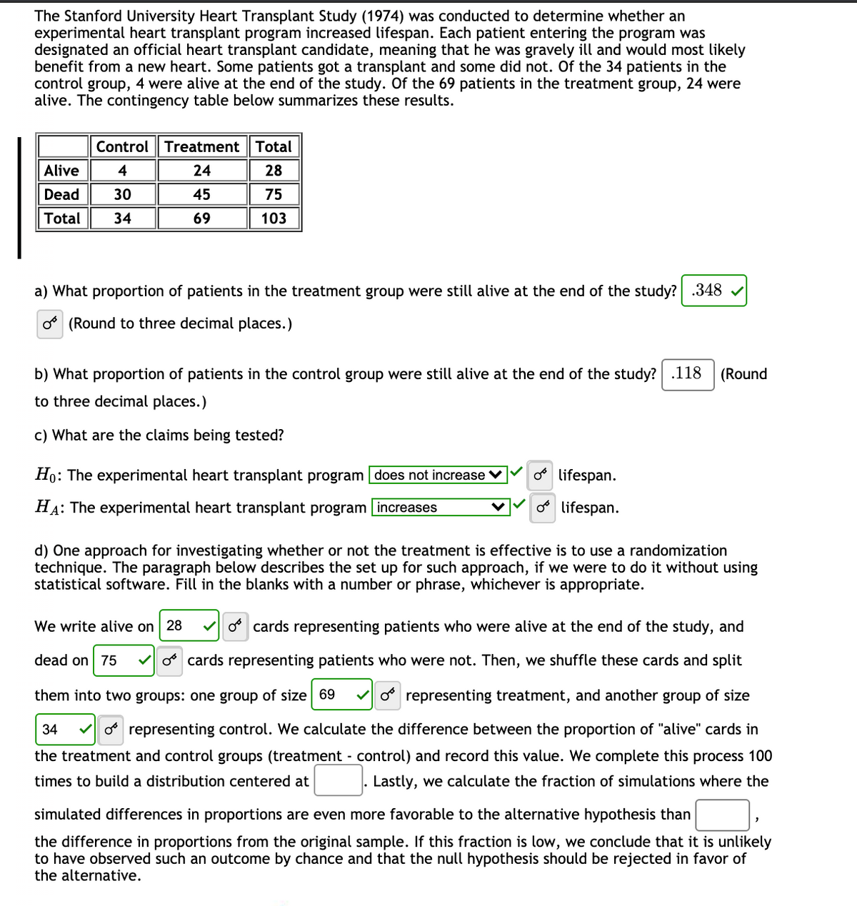
The Stanford University Heart Transplant Study (1974) was conducted to determine whether an experimental heart transplant program increased lifespan. Each patient entering the program was designated an official heart transplant candidate, meaning that he was gravely ill and would most likely benefit from a new heart. Some patients got a transplant and some did not. Of the 34 patients in the control group, 4 were alive at the end of the study. Of the 69 patients in the treatment group, 24 were alive. The contingency table below summarizes these results.

	Control	Treatment	Total
Alive	4	24	28
Dead	30	45	75
Total	34	69	103

a) What proportion of patients in the treatment group were still alive at the end of the study? .348Correct (Round to three decimal places.)

b) What proportion of patients in the control group were still alive at the end of the study? .118 (Round to three decimal places.)

c) What are the claims being tested?

H0H0: The experimental heart transplant program Select an answer increases does not increase Correct lifespan.
HAHA: The experimental heart transplant program Select an answer increases does not increase Correct lifespan.

d) One approach for investigating whether or not the treatment is effective is to use a randomization technique. The paragraph below describes the set up for such approach, if we were to do it without using statistical software. Fill in the blanks with a number or phrase, whichever is appropriate.

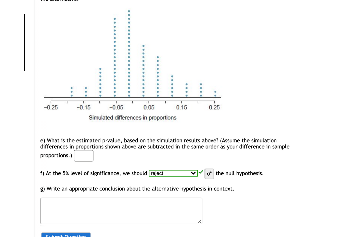
We write alive on Correct cards representing patients who were alive at the end of the study, and dead on Correct cards representing patients who were not. Then, we shuffle these cards and split them into two groups: one group of size Correct representing treatment, and another group of size Correct representing control. We calculate the difference between the proportion of "alive" cards in the treatment and control groups (treatment - control) and record this value. We complete this process 100 times to build a distribution centered at _____?Lastly, we calculate the fraction of simulations where the simulated differences in proportions are even more favorable to the alternative hypothesis than________? the difference in proportions from the original sample. If this fraction is low, we conclude that it is unlikely to have observed such an outcome by chance and that the null hypothesis should be rejected in favor of the alternative.

e) What is the estimated p-value, based on the simulation results above? (Assume the simulation differences in proportions shown above are subtracted in the same order as your difference in sample proportions.)

g) Write an appropriate conclusion about the alternative hypothesis in context.

The Stanford University Heart Transplant Study (1974) was conducted to determine whether an
experimental heart transplant program increased lifespan. Each patient entering the program was
designated an official heart transplant candidate, meaning that he was gravely ill and would most likely
benefit from a new heart. Some patients got a transplant and some did not. Of the 34 patients in the
control group, 4 were alive at the end of the study. Of the 69 patients in the treatment group, 24 were
alive. The contingency table below summarizes these results.
Control Treatment
Total
Alive
4
24
28
Dead
30
45
75
Total
34
69
103
a) What proportion of patients in the treatment group were still alive at the end of the study? .348 v
o (Round to three decimal places.)
b) What proportion of patients in the control group were still alive at the end of the study? .118
(Round
to three decimal places.)
c) What are the claims being tested?
Ho: The experimental heart transplant program does not increase V
o lifespan.
HA: The experimental heart transplant program increases
o lifespan.
d) One approach for investigating whether or not the treatment is effective is to use a randomization
technique. The paragraph below describes the set up for such approach, if we were to do it without using
statistical software. Fill in the blanks with a number or phrase, whichever is appropriate.
We write alive on 28
o cards representing patients who were alive at the end of the study, and
dead on 75
o cards representing patients who were not. Then, we shuffle these cards and split
them into two groups: one group of size 69
V o representing treatment, and another group of size
34
o representing control. We calculate the difference between the proportion of "alive" cards in
the treatment and control groups (treatment - control) and record this value. We complete this process 100
times to build a distribution centered at
Lastly, we calculate the fraction of simulations where the
simulated differences in proportions are even more favorable to the alternative hypothesis than
the difference in proportions from the original sample. If this fraction is low, we conclude that it is unlikely
to have observed such an outcome by chance and that the null hypothesis should be rejected in favor of
the alternative.

-0.25
-0.15
-0.05
0.05
0.15
0.25
Simulated differences in proportions
e) What is the estimated p-value, based on the simulation results above? (Assume the simulation
differences in proportions shown above are subtracted in the same order as your difference in sample
proportions.)
f) At the 5% level of significance, we should reject
o the null hypothesis.
g) Write an appropriate conclusion about the alternative hypothesis in context.
Submit Ouoction
.......

Expert Solution

Trending now

This is a popular solution!

Step by step

Solved in 4 steps with 1 images

SEE SOLUTION Check out a sample Q&A here

Knowledge Booster

$Data Collection, Sampling Methods, and Bias$

Learn more about

Need a deep-dive on the concept behind this application? Look no further. Learn more about this topic, statistics and related others by exploring similar questions and additional content below.