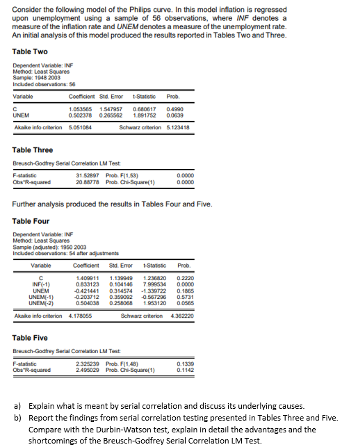
Consider the following model of the Philips curve. In this model inflation is regressedupon unemployment using a sample of 56 observations, where INF denotes ameasure of the inflation rate and UNEM denotes a measure of the unemployment rate.An initial analysis of this model produced the results reported in Tables Two and Three.Table TwoDependent Variable: INFMethod: Least SquaresSample: 1948 2003Included observations: 56VariableCoefficient Std. Errort-StatisticProb.0.49900.06391.053565 1.5479570.6806171.891752UNEM0.502378 0.265562Akaike info criterion 5.051084Schwarz criterion 5.123418Table ThreeBreusch-Godtrey Serial Correlation LM TestF-statistic31.52897 Prob. F(1,53)20.88778 Prob. Chi-Square(1)0.0000Obs'R-squared0.0000Further analysis produced the results in Tables Four and Five.Table FourDependent Variable: INFMethod: Least SquaresSample (adusted) 1950 2003Included observations: 54 after adjustmentsVariableCoefficientStd. Errort-StatisticProb.1.4099110.833123-0.421441-0.2037 120.5040381.1399490.1041460.3145740.3590920 2580681.236820INF(-1)UNEMUNEM(-1)UNEMI-2)7.999534-1.339722-0.5672961.9531200.22200.00000.18650.57310.0565Akaike info criterion 4.178055Schwarz ariterion4.362220Table FiveBreusch-Godfrey Serial Correlation LM TestF-statisticObs'R-squared2.325239 Prob. F(1,48)2495029 Prob. Chi-Square(1)0.13390.1142a) Explain what is meant by serial correlation and discuss its underlying causes.b) Report the findings from serial correlation testing presented in Tables Three and Five.Compare with the Durbin-Watson test, explain in detail the advantages and theshortcomings of the Breusch-Godfrey Serial Correlation LM Test.

a) Serial correlation: Serial correlation is the correlation between the variable and its lagged…

Answered: Consider the following model of the…

College Algebra

7th Edition

ISBN:9781305115545

Author:James Stewart, Lothar Redlin, Saleem Watson

Publisher:James Stewart, Lothar Redlin, Saleem Watson

Chapter1: Equations And Graphs

Section: Chapter Questions

Problem 10T: Olympic Pole Vault The graph in Figure 7 indicates that in recent years the winning Olympic men’s...

See similar textbooks

Similar questions

Olympic Pole Vault The graph in Figure 7 indicates that in recent years the winning Olympic men’s pole vault height has fallen below the value predicted by the regression line in Example 2. This might have occurred because when the pole vault was a new event there was much room for improvement in vaulters’ performances, whereas now even the best training can produce only incremental advances. Let’s see whether concentrating on more recent results gives a better predictor of future records. (a) Use the data in Table 2 (page 176) to complete the table of winning pole vault heights shown in the margin. (Note that we are using x=0 to correspond to the year 1972, where this restricted data set begins.) (b) Find the regression line for the data in part ‚(a). (c) Plot the data and the regression line on the same axes. Does the regression line seem to provide a good model for the data? (d) What does the regression line predict as the winning pole vault height for the 2012 Olympics? Compare this predicted value to the actual 2012 winning height of 5.97 m, as described on page 177. Has this new regression line provided a better prediction than the line in Example 2?
Find the curve of best-fit y = axb to the following data by using the method of least square.
An econometrician suspects that the residuals of her model might be autocorrelated. Explain the steps involved in testing this theory using the Durbin–Watson (DW) test
A researcher notes that, in a certain region, a disproportionate number of software millionaires were born around the year 1955. Is this a coincidence, or does birth year matter when gauging whether a software founder will besuccessful? The researcher investigated this question by analyzing the data shown in the accompanying table. Complete parts a through c below. a. Find the coefficient of determination for the simple linear regression model relating number (y) of software millionaire birthdays in a decade to total number (x) of births in the region. Interpret the result. The coefficient of determination is 1.___? (Round to three decimal places as needed.) This value indicates that 2.____ of the sample variation in the number of software millionaire birthdays is explained by the linear relationship with the total number of births in the region. (Round to one decimal place as needed.) b. Find the coefficient of determination for the simple linear regression model…
Compute the forecasted values for Yt for July and August in 2020 by using the modelsstated in (c) and (d)
Based on the EViews results above, answer the following questions.a. What is your comments on the diagnostic tests of the model? i. Autocorrelation test ii. Heteroscedasticity test iii. Normality
Which of the following is NOT CORRECT? A) The past purchase frequency (freqi) affects the purchase probability positively – i.e., customers with high past purchase frequency are more likely to purchase our product in the next year than those with low past purchase frequency. B) In general, customers are likely to buy our product because the baseline parameter is negative. C) High-income customers are more likely to purchase our product in the next year than low- income customers because the coefficient corresponding to the income variable (incomei) is positive. D) Although the number of flyers (nmaili) positively affects the purchase probability, it is not guaranteed that sending flyers to customers as many as possible maximizes profits.
Table 14.17 The Least Squares Point Estimates for Exercise 14.51 Bo = 10.3676 (.3710) B1 = .0500 (<.001) B2 = 6.3218 (.0152) B3 = -11.1032 (.0635) B4 = -.4319 (.0002) Questions Using the t statistic and appropriate critical values, test Ho: βj = 0 versus Ha: βj ≠ 0 by setting α equal to .05. Which independent variables are significantly related to y in the model with α = .05? Using the t statistic and appropriate critical values, test Ho: βj = 0 versus Ha: βj ≠ 0 by setting α equal to .01. Which independent variables are significantly related to y in the model with α = .01? Find the p-value for testing Ho: βj = 0 versus Ha: βj ≠ 0 on the output. Using the p-value, determine whether we can reject Ho by setting α equal to .10, .05, .01, and .001. What do you conclude about the significance of the independent variables in the model? Calculate the 95 percent confidence interval for βj. Discuss one practical application of this interval. Calculate the 99 percent confidence interval for…
The following table shows the length, in centimeters, of the humerus and the total wingspan, in centimeters, of several pterosaurs, which are extinct flying reptiles. (A graphing calculator is recommended.) (a) Find the equation of the least-squares regression line for the data. (Where × is the independent variable.) Round constants to the nearest hundredth. y= ? (b) Use the equation from part (a) to determine, to the nearest centimeter, the projected wingspan of a pterosaur if its humerus is 52 centimeters. ? cm
Suppose a study wants to predict the market price of a certain species of turtle (Y) based on the following independent variables indicated in the table. Based from the table, what is the equation of the multiple linear regression? (Round off up to two decimal places. Market Price = 0.07 - 0.40*weight + 1.51*length + 1.41*width + 0.80*age Market Price = - 0.40*weight + 1.51*length + 1.41*width + 0.80*age Market Price = 0.07 + 0.40*weight + 1.51*length + 1.41*width + 0.80*age Market Price = 0.07 - 0.40 + weight + 1.51 + length + 1.41 + width + 0.80 + age
The following table shows the annual number of PhD graduates in a country in various fields. NaturalSciences Engineering SocialSciences Education 1990 70 10 70 30 1995 130 40 110 50 2000 330 130 280 140 2005 490 370 460 210 2010 590 550 830 520 2012 690 590 1,000 900 (a) With x = the number of social science doctorates and y = the number of education doctorates, use technology to obtain the regression equation. (Round coefficients to three significant digits.) y(x) = Graph the associated points and regression line. (b) What does the slope tell you about the relationship between the number of social science doctorates and the number of education doctorates? The slope tells us the increase in the number of social science doctorates for each additional education doctorate.The slope tells us the increase in the number of education doctorates for each additional social science doctorate. The slope tells us the decrease in the number…
The following table shows the annual number of PhD graduates in a country in various fields. NaturalSciences Engineering SocialSciences Education 1990 70 10 60 30 1995 130 40 120 50 2000 330 130 280 140 2005 490 370 460 210 2010 590 550 830 520 2012 690 590 1,000 900 (a) With x = the number of social science doctorates and y = the number of education doctorates, use technology to obtain the regression equation. (Round coefficients to three significant digits.) y(x) = Graph the associated points and regression line. (b) What does the slope tell you about the relationship between the number of social science doctorates and the number of education doctorates? The slope tells us the increase in the number of education doctorates for each additional social science doctorate.The slope tells us the decrease in the number of education doctorates for each additional social science doctorate. The slope tells us the increase in the number…

SEE MORE QUESTIONS

Recommended textbooks for you

College Algebra

Algebra

ISBN:

9781305115545

Author:

James Stewart, Lothar Redlin, Saleem Watson

Publisher:

Cengage Learning

Linear Algebra: A Modern Introduction

Algebra

ISBN:

9781285463247

Author:

David Poole

Publisher:

Cengage Learning

Algebra & Trigonometry with Analytic Geometry

Algebra

ISBN:

9781133382119

Author:

Swokowski

Publisher:

Cengage

College Algebra

Algebra

ISBN:

9781305115545

Author:

James Stewart, Lothar Redlin, Saleem Watson

Publisher:

Cengage Learning

Linear Algebra: A Modern Introduction

Algebra

ISBN:

9781285463247

Author:

David Poole

Publisher:

Cengage Learning

Algebra & Trigonometry with Analytic Geometry

Algebra

ISBN:

9781133382119

Author:

Swokowski

Publisher:

Cengage

SEE MORE TEXTBOOKS