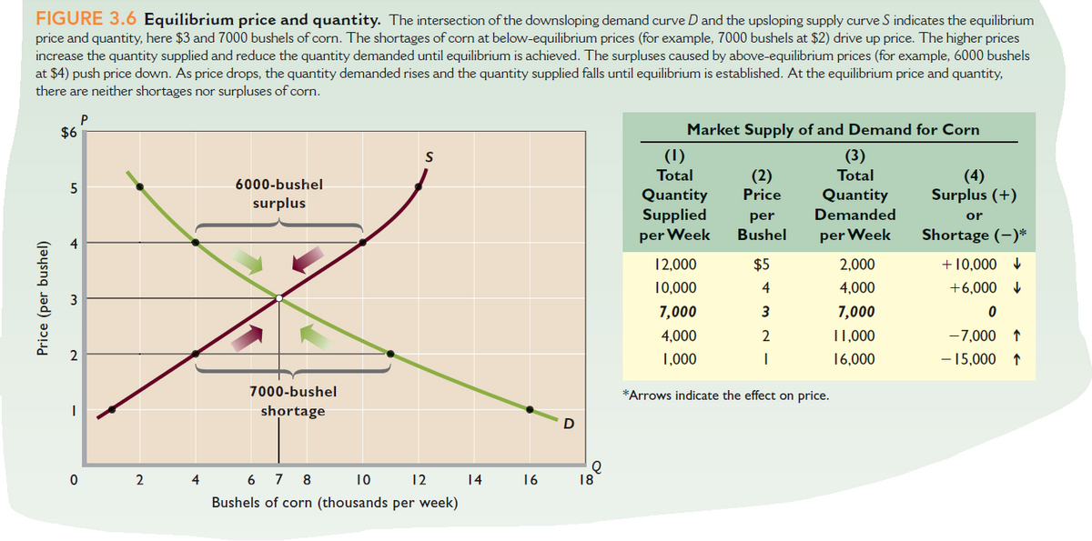
FIGURE 3.6 Equilibrium price and quantity. The intersection of the downsloping demand curve D and the upsloping supply curve S indicates the equilibrium price and quantity, here $3 and 7000 bushels of corn. The shortages of corn at below-equilibrium prices (for example, 7000 bushels at $2) drive up price. The higher prices increase the quantity supplied and reduce the quantity demanded until equilibrium is achieved. The surpluses caused by above-equilibrium prices (for example, 6000 bushels at $4) push price down. As price drops, the quantity demanded rises and the quantity supplied falls until equilibrium is established. At the equilibrium price and quantity, there are neither shortages nor surpluses of corn. $6 Market Supply of and Demand for Corn (1) (3) Total S Total (2) Price (4) Surplus (+) 5 6000-bushel Quantity Supplied per Week Quantity surplus per Demanded or Bushel per Week Shortage (-)* 12,000 $5 2,000 +10,000 V 10,000 4 4,000 +6,000 7,000 7,000 4,000 2 11,000 -7,000 1,000 16,000 - 15,000 ↑ 7000-bushel *Arrows indicate the effect on price. shortage 2 4 6 7 8 10 12 14 16 18 Bushels of corn (thousands per week) Price (per bushel)
FIGURE 3.6 Equilibrium price and quantity. The intersection of the downsloping demand curve D and the upsloping supply curve S indicates the equilibrium price and quantity, here $3 and 7000 bushels of corn. The shortages of corn at below-equilibrium prices (for example, 7000 bushels at $2) drive up price. The higher prices increase the quantity supplied and reduce the quantity demanded until equilibrium is achieved. The surpluses caused by above-equilibrium prices (for example, 6000 bushels at $4) push price down. As price drops, the quantity demanded rises and the quantity supplied falls until equilibrium is established. At the equilibrium price and quantity, there are neither shortages nor surpluses of corn. $6 Market Supply of and Demand for Corn (1) (3) Total S Total (2) Price (4) Surplus (+) 5 6000-bushel Quantity Supplied per Week Quantity surplus per Demanded or Bushel per Week Shortage (-)* 12,000 $5 2,000 +10,000 V 10,000 4 4,000 +6,000 7,000 7,000 4,000 2 11,000 -7,000 1,000 16,000 - 15,000 ↑ 7000-bushel *Arrows indicate the effect on price. shortage 2 4 6 7 8 10 12 14 16 18 Bushels of corn (thousands per week) Price (per bushel)

Principles of Microeconomics (MindTap Course List)
8th Edition
ISBN:9781305971493
Author:N. Gregory Mankiw
Publisher:N. Gregory Mankiw
Chapter7: Consumers, Producers, And The Efficiency Of Markets
Section: Chapter Questions
Problem 9PA

Related questions
Question
Refer to Figure 3.6, page 55. Assume that the graph depicts the U.S. domestic market for corn. How many bushels of corn, if any, will the United States export or import at a world price of $1, $2, $3, $4, and $5? Use this information to construct the U.S. export supply curve and import
Transcribed Image Text:FIGURE 3.6 Equilibrium price and quantity. The intersection of the downsloping demand curve D and the upsloping supply curve S indicates the equilibrium
price and quantity, here $3 and 7000 bushels of corn. The shortages of corn at below-equilibrium prices (for example, 7000 bushels at $2) drive up price. The higher prices
increase the quantity supplied and reduce the quantity demanded until equilibrium is achieved. The surpluses caused by above-equilibrium prices (for example, 6000 bushels
at $4) push price down. As price drops, the quantity demanded rises and the quantity supplied falls until equilibrium is established. At the equilibrium price and quantity,
there are neither shortages nor surpluses of corn.
$6
Market Supply of and Demand for Corn
(1)
(3)
Total
S
Total
(2)
Price
(4)
Surplus (+)
5
6000-bushel
Quantity
Supplied
per Week
Quantity
surplus
per
Demanded
or
Bushel
per Week
Shortage (-)*
12,000
$5
2,000
+10,000 V
10,000
4
4,000
+6,000
7,000
7,000
4,000
2
11,000
-7,000
1,000
16,000
- 15,000 ↑
7000-bushel
*Arrows indicate the effect on price.
shortage
2
4
6
7
8
10
12
14
16
18
Bushels of corn (thousands per week)
Price (per bushel)
Expert Solution
This question has been solved!
Explore an expertly crafted, step-by-step solution for a thorough understanding of key concepts.

This is a popular solution!

Trending now
This is a popular solution!

Step by step
Solved in 4 steps with 1 images

Knowledge Booster


Learn more about
Need a deep-dive on the concept behind this application? Look no further. Learn more about this topic, economics and related others by exploring similar questions and additional content below.Recommended textbooks for you
Principles of Microeconomics (MindTap Course List)
Economics
ISBN:
9781305971493
Author:
N. Gregory Mankiw
Publisher:
Cengage Learning

Principles of Macroeconomics (MindTap Course List)
Economics
ISBN:
9781285165912
Author:
N. Gregory Mankiw
Publisher:
Cengage Learning

Essentials of Economics (MindTap Course List)
Economics
ISBN:
9781337091992
Author:
N. Gregory Mankiw
Publisher:
Cengage Learning
Principles of Microeconomics (MindTap Course List)
Economics
ISBN:
9781305971493
Author:
N. Gregory Mankiw
Publisher:
Cengage Learning
Principles of Macroeconomics (MindTap Course List)
Economics
ISBN:
9781285165912
Author:
N. Gregory Mankiw
Publisher:
Cengage Learning
Essentials of Economics (MindTap Course List)
Economics
ISBN:
9781337091992
Author:
N. Gregory Mankiw
Publisher:
Cengage Learning

Principles of Economics (MindTap Course List)
Economics
ISBN:
9781305585126
Author:
N. Gregory Mankiw
Publisher:
Cengage Learning

Principles of Economics, 7th Edition (MindTap Cou…
Economics
ISBN:
9781285165875
Author:
N. Gregory Mankiw
Publisher:
Cengage Learning