Let x be a random variable that represents the batting average of a professional baseball player. Let y be a random variable that represents the percentage of strikeouts of a professional baseball player. A random sample of n = 6 professional baseball players gave the following information. x 0.312 3.4 0.367 3.1 0.269 11.1 0.300 0.340 4.0 0.248 8.6 7.5 (a) Verify that Ex = 1.836, Ey = 37.7, Ex² = 0.571498, Ey2 = 290.59, Exy = 10.9272, and r= -0.845. Ex 1.836 Ly 37.7 Ex2 0.571498 Ey2 290.59 Exy 10.9272 r -0.845 (b) Use a 5% level of significance to test the claim that p + 0. (Use 2 decimal places.) t-3.16 critical t + 2.776 Conclusion Reject the null hypothesis, there is sufficient evidence that p differs from 0. Reject the null hypothesis, there is insufficient evidence that p differs from 0. O Fail to reject the null hypothesis, there is insufficient evidence that p differs from 0. Fail to reject the null hypothesis, there is sufficient evidence that p differs from 0. (c) Verify that S, 1.9623, a 25.531, and b = -62.900. Se 1.9623 a 25.531 b -62.900
Let x be a random variable that represents the batting average of a professional baseball player. Let y be a random variable that represents the percentage of strikeouts of a professional baseball player. A random sample of n = 6 professional baseball players gave the following information. x 0.312 3.4 0.367 3.1 0.269 11.1 0.300 0.340 4.0 0.248 8.6 7.5 (a) Verify that Ex = 1.836, Ey = 37.7, Ex² = 0.571498, Ey2 = 290.59, Exy = 10.9272, and r= -0.845. Ex 1.836 Ly 37.7 Ex2 0.571498 Ey2 290.59 Exy 10.9272 r -0.845 (b) Use a 5% level of significance to test the claim that p + 0. (Use 2 decimal places.) t-3.16 critical t + 2.776 Conclusion Reject the null hypothesis, there is sufficient evidence that p differs from 0. Reject the null hypothesis, there is insufficient evidence that p differs from 0. O Fail to reject the null hypothesis, there is insufficient evidence that p differs from 0. Fail to reject the null hypothesis, there is sufficient evidence that p differs from 0. (c) Verify that S, 1.9623, a 25.531, and b = -62.900. Se 1.9623 a 25.531 b -62.900

MATLAB: An Introduction with Applications
6th Edition
ISBN:9781119256830
Author:Amos Gilat
Publisher:Amos Gilat
Chapter1: Starting With Matlab
Section: Chapter Questions
Problem 1P

Related questions
Question
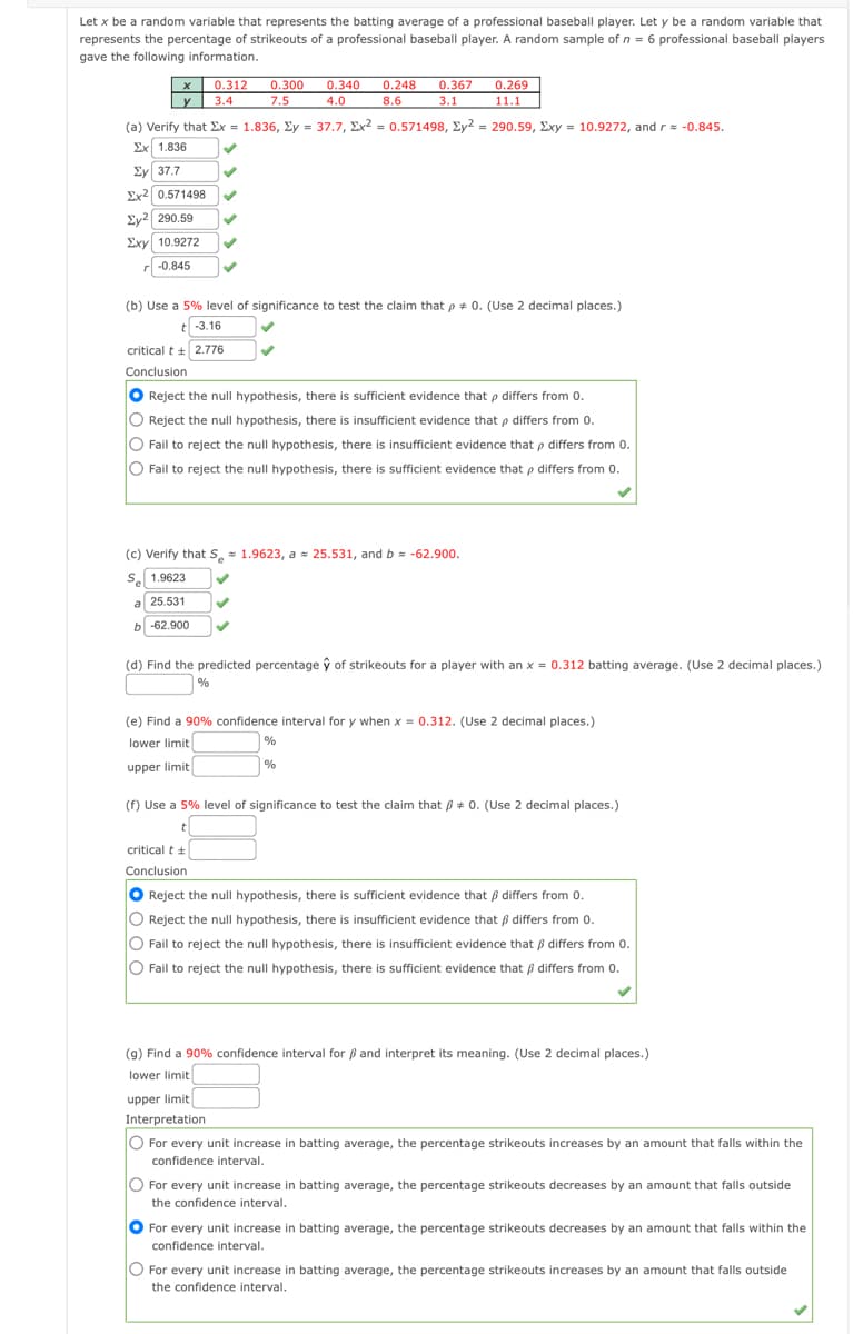
Transcribed Image Text:Let x be a random variable that represents the batting average of a professional baseball player. Let y be a random variable that
represents the percentage of strikeouts of a professional baseball player. A random sample of n = 6 professional baseball players
gave the following information.
х
0.312
y 3.4
0.300
7.5
0.340
0.248
0.367
3.1
0.269
4.0
8.6
11.1
(a) Verify that Ex = 1.836, Ey = 37.7, Ex2 = 0.571498, Ey2 = 290.59, Exy = 10.9272, andr= -0.845.
Ex 1.836
Ey 37.7
Ex2 0.571498
Ey2 290.59
Exy 10.9272
r -0.845
(b) Use a 5% level of significance to test the claim that p + 0. (Use 2 decimal places.)
t -3.16
critical t + 2.776
Conclusion
O Reject the null hypothesis, there is sufficient evidence that p differs from 0.
O Reject the null hypothesis, there is insufficient evidence that p differs from 0.
O Fail to reject the null hypothesis, there is insufficient evidence that p differs from 0.
O Fail to reject the null hypothesis, there is sufficient evidence that p differs from 0.
(c) Verify that S, 1.9623, a = 25.531, and b -62.900.
Se 1.9623
a 25.531
b -62.900
(d) Find the predicted percentage ŷ of strikeouts for a player with an x = 0.312 batting average. (Use 2 decimal places.)
| %
(e) Find a 90% confidence interval for y when x = 0.312. (Use 2 decimal places.)
lower limit
%
upper limit
%
(f) Use a 5% level of significance to test the claim that B + 0. (Use 2 decimal places.)
critical t +
Conclusion
O Reject the null hypothesis, there is sufficient evidence that ß differs from 0.
O
Reject the null hypothesis, there is insufficient evidence that ß differs from 0.
O Fail to reject the null hypothesis, there is insufficient evidence that B differs from 0.
O Fail to reject the null hypothesis, there is sufficient evidence that ß differs from 0.
(g) Find a 90% confidence interval for ß and interpret its meaning. (Use 2 decimal places.)
lower limit
upper limit
Interpretation
O For every unit increase in batting average, the percentage strikeouts increases by an amount that falls within the
confidence interval.
O For every unit increase in batting average, the percentage strikeouts decreases by an amount that falls outside
the confidence interval.
For every unit increase in batting average, the percentage strikeouts decreases by an amount that falls within the
confidence interval.
O For every unit increase in batting average, the percentage strikeouts increases by an amount that falls outside
the confidence interval.
Expert Solution
This question has been solved!
Explore an expertly crafted, step-by-step solution for a thorough understanding of key concepts.

Step by step
Solved in 5 steps

Recommended textbooks for you
MATLAB: An Introduction with Applications
Statistics
ISBN:
9781119256830
Author:
Amos Gilat
Publisher:
John Wiley & Sons Inc

Probability and Statistics for Engineering and th…
Statistics
ISBN:
9781305251809
Author:
Jay L. Devore
Publisher:
Cengage Learning

Statistics for The Behavioral Sciences (MindTap C…
Statistics
ISBN:
9781305504912
Author:
Frederick J Gravetter, Larry B. Wallnau
Publisher:
Cengage Learning
MATLAB: An Introduction with Applications
Statistics
ISBN:
9781119256830
Author:
Amos Gilat
Publisher:
John Wiley & Sons Inc
Probability and Statistics for Engineering and th…
Statistics
ISBN:
9781305251809
Author:
Jay L. Devore
Publisher:
Cengage Learning
Statistics for The Behavioral Sciences (MindTap C…
Statistics
ISBN:
9781305504912
Author:
Frederick J Gravetter, Larry B. Wallnau
Publisher:
Cengage Learning

Elementary Statistics: Picturing the World (7th E…
Statistics
ISBN:
9780134683416
Author:
Ron Larson, Betsy Farber
Publisher:
PEARSON

The Basic Practice of Statistics
Statistics
ISBN:
9781319042578
Author:
David S. Moore, William I. Notz, Michael A. Fligner
Publisher:
W. H. Freeman

Introduction to the Practice of Statistics
Statistics
ISBN:
9781319013387
Author:
David S. Moore, George P. McCabe, Bruce A. Craig
Publisher:
W. H. Freeman