UESTION 4 - problem-type question requiring detailed written answers. he members of a sports club were concerned about the effect of the weather on e outcome of their cricket matches. The results for the 75 matches played were corded in the following table: Results Win Draw Lose TOTAL Good 17 9 7 33 Weather Bad 9 10 23 52 TOTAL 26 19 30 75 If a match was selected at random, what is the probability that: (a) The sports club did not draw the match. (b) The weather was good and the club at draw the match. (c) The club lost the match given that the weather was bad. (d) The weather was good or the sports club win the match. (e) Are the events "Win" and "Lose" the match, mutually exclusive events. Us the rules of probabilities to justify your answer.
UESTION 4 - problem-type question requiring detailed written answers. he members of a sports club were concerned about the effect of the weather on e outcome of their cricket matches. The results for the 75 matches played were corded in the following table: Results Win Draw Lose TOTAL Good 17 9 7 33 Weather Bad 9 10 23 52 TOTAL 26 19 30 75 If a match was selected at random, what is the probability that: (a) The sports club did not draw the match. (b) The weather was good and the club at draw the match. (c) The club lost the match given that the weather was bad. (d) The weather was good or the sports club win the match. (e) Are the events "Win" and "Lose" the match, mutually exclusive events. Us the rules of probabilities to justify your answer.

MATLAB: An Introduction with Applications
6th Edition
ISBN:9781119256830
Author:Amos Gilat
Publisher:Amos Gilat
Chapter1: Starting With Matlab
Section: Chapter Questions
Problem 1P

Related questions
Question
100%
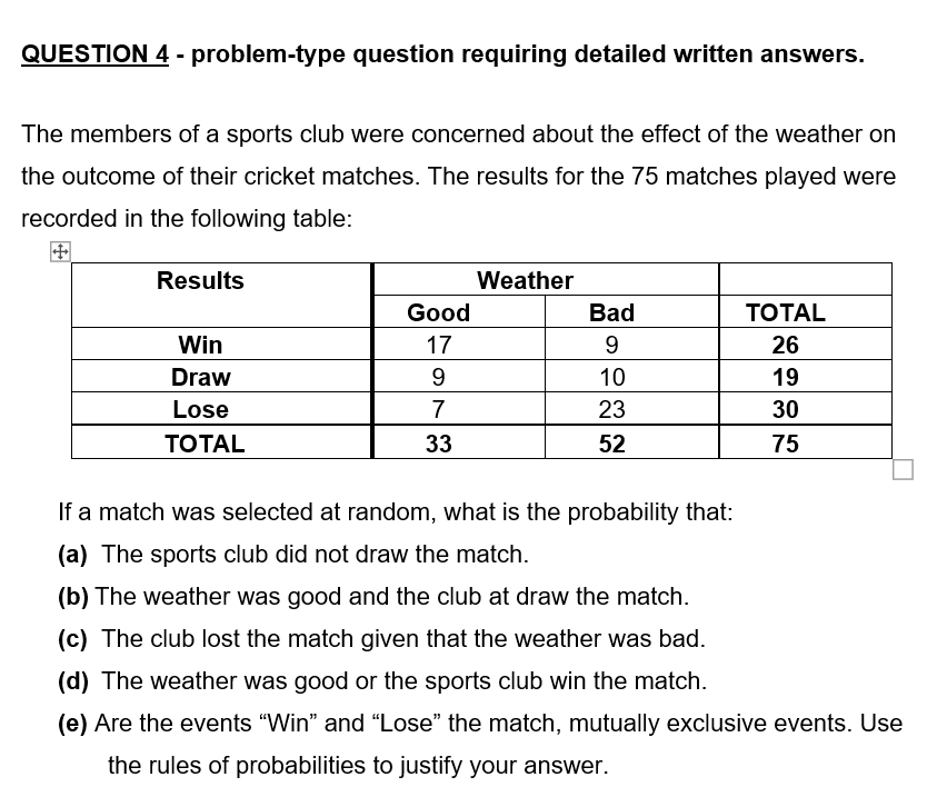
Transcribed Image Text:QUESTION 4 - problem-type question requiring detailed written answers.
The members of a sports club were concerned about the effect of the weather on
the outcome of their cricket matches. The results for the 75 matches played were
recorded in the following table:
Results
Win
Draw
Lose
TOTAL
Good
17
9
7
33
Weather
Bad
9
10
23
52
If a match was selected at random, what is the probability that:
(a) The sports club did not draw the match.
(b) The weather was good and the club at draw the match.
(c) The club lost the match given that the weather was bad.
(d) The weather was good or the sports club win the match.
TOTAL
26
19
30
75
(e) Are the events "Win" and "Lose" the match, mutually exclusive events. Use
the rules of probabilities to justify your answer.
Transcribed Image Text:z
0.0
0.1
0.2
0.3
0.4
0.5
0.6
0.7
0.8
0.9
1.0
1.1
1.2
1.3
1.5
1.6
1.7
1.8
20
2.1
2.2
2.3
2.4
2.5
2.6
2.7
2.8
2.9
3.0
5000
5398
5793
6179
3.2
3.3
6554
6915
7257
7580
7881
8159
8413
8643
8849
9032
9192
9332
9452
9554
9641
9713
9772
9821
9861
9893
9918
9938
9953
9965
9981
9987
00
-3.4 0003
0005
-3.2
0007
-3.1 0010
-3.0
-2.9 0019
-2.8 0026
-2.7 0035
0047
-2.5 0062
01
5040
5438
5832
6217
-14 0808
-1.3 0968
-1.2 1151
-1.1 1357
-1.0 1587
6591
6950
-0.9 1841
-0.8 2119
-0.7 2420
-0.6 2743
-0.5
7291
7611
7910
8186
8438
-0.4 3446
-0.3 3821
-0.2 4207
-0.1
0.01 5000
8665
8869
9049
9207
9345
9990
9993
9995
9997
This is Table IV of Appendix C.
9463
9564
9649
9719
9778
9826
9864
9896
9920
9940
9955
9966
9975
9982
9987
9991
9993
9995
9997
01
0003
0005
0007
0009
0013
-1.9 0287 0281
-1.8 0359
-1.7 0446
0018
0025
0034
0045
0060
-1.6 0548 0537
-1.5 0668
0655
0351
0436
0793
0951
1131
1335
1562
1814
2090
2389
2709
3050
3409
3783
102
4168
5080
4960
5478
5871
6255
6628
6985
7324
7642
7939
8212
8461
8686
8888
0082 0080
0078
0132
-2.3 0107 0104 0102
-2.2 0139
-21
-2.0 0228
0136
0174
0179
0170
0222
0217
9066
9222
9357
9474
9573
9656
9726
9783
9830
9868
9898
Table IV Standard Normal Distribution Table
9922
9941
9956
9967
9976
9982
9987
9991
9994
9995
9997
1002
0001
0005
0006
0009
0018
0024
0033
0044
0059
0274
0344
0427
0526
0643
0778
0934
1112
1314
1539
1788
2061
2358
2676
3372
3745
4522
4920
003
5120
5517
5910
6293
6664
7019
7357
7673
7967
8238
8485
8708
8907
9082
9236
9370
9484
9582
P(1) ---
xC₂
Poisson probability formala P(x)
9834
9871
9901
9925
9943
9957
9968
9977
9495
9591
9664
9671
9732 9738
9788
9793
9983
9988
9991
9994
9996
9997
normal curve to the left of z with the
values of z equal to 0 or positive.
03
0003
0004
0006
0009
0012
0017
0023
0032
0043
0057
0075
0099
0129
0166
0212
0268
0336
0418
0516
0630
0764
0918
1093
1292
1515
1762
2033
2327
3336
3707
4483
4880
Joint probability of two mutually exclusive events:
PA and B) 0
. Addition rule for mutually nonexclusive events:
P(AB)=P(A) + P(B)- PA and B)
Addition rule for mutually exclusive events:
P(AB)=P(A) + P(B)
Chapter 5. Discrete Random Variables and Their
Probability Distributions
Mean of a discrete random variable x:=xP(x)
. Standard deviation of a discrete random variable x:
a-√2+¹P(1)-²
04
5160
5557
5948
6331
Chapter 6. Continuous Random Variables
and the Normal Distribution
2 value for an x value
Value of x when . o, and are known: x=+50
7054
Chapter 7. Sampling Distributions
- Mean of :
. Standard deviation of I when n/Ns .05 aya/V
I-K
7389
7704
7995
8264
8508
8729
8925
9099
9251
factorial: w-1-2) 3-2-1
Number of combinations of a items selected x at a time:
F.x-x)
. Number of permutations of items selected x at a time:
04
0003
0004
0006
0008
0012
(-x)
Binomial probability formulac P(x)-C, pq
Mean and standard deviation of the binomial distribution:
panday
Hypergeometric probability formula:
9959
9969
9977
9984
0016
0023
0031
0041
0055
9992
9994
9996
9997
0073
0096
0125
xt
. Mean, variance, and standard deviation of the Poisson prob
ability distribution:
=A²A, and VĀ
0207
0262
0329
0409
0505
0618
0749
0901
1075
1271
1492
2005
2296
2611
3300
3669
The entries in this table give the
cumulative area under the standard
normal curve to the left of z with the
values of z equal to 0 or negative.
4443
9838
9842
9875 9878
9904
9906
9927
9945
4840
005
5199
5596
5987
6368
6736
7088
7422
7734
8023
8289
8531
9505
9599
9678
9744
9798
9929
9946
9960
9970
8749
8770
8944
8962
9115 9131
9265
9279
9394
9406
9984
9989
9992
9994
9996
9997
05
0003
0004
0006
0008
0011
0016
0022
0030
0040
0054
0071
0094
0122
0158
0202
0256
0322
0401
0495
0606
0735
0885
1056
1251
1469
1711
1977
2266
2578
2912
3264
3632
06
5239
4404
4801
56.36
6026
6406
6772
7123
7454
7764
8051
9515
9608
8315
8340
8554 8577
9686
9750
9803
9961
9971
9985
9992
9994
9996
9997
06
9846
9850
9881
9884
9909
9911
9931
9932
9945 9949
0003
0004
0006
000
0011
0015
0021
0039
0052
0091
0119
0197
0250
0314
0392
0485
0594
0721
0869
1038
1446
1685
1949
2236
2546
3228
3594
4364
1867
5279
3675
6064
6443
4761
7157
746
7794
8078
of
8980
9147
9292
9418
9525
9616
9693
9756
9808
9962
9972
9979
9985
9995
9996
9997
107
0003
0004
0005
0008
0011
0015
0021
0028
0038
0051
0089
0116
0150
0192
0244
0307
0384
0475
0582
0708
0853
1020
1423
3192
3557
108
08
5319
5714
6103
6480
7190
7517
7823
8106
8365
8599
- Margin of error of the estimate for a
E20 of th
- Determining sample size for estimating
8810
8997
9162
9306
9429
9535
9625
9854
9913
9934
9951
9963
9973
9956
0003
0004
0005
0007
9699
9706
9761 9767
9812
9993
9995
9996
0014
0020
where=1/Ö
0037
0049
0066
0087
0113
0146
0188
0239
0301
0375
pt 2 where
Margin of error of the estimate for p
E-2 where - V
Determining sample size for estimating p
-²/E²
0465
0571
0694
0838
1003
1401
4681
5359
5753
6141
6517
6879
7549
8133
8389
8830
9015
Confidence interval for p for a large sample:
V/n
9177
9319
9545
Chapter 9- Hypothesis Tests about the Mean
and Proportion
9857
9890
9916
9936
9952
9964
9986
9990
9993
9995
9997
9998
09
0002
0003
0005
0007
0010
1660
1635
1922
1894
2206
2177 2148
2514
2483 2451
2843 2810 2776
0019
0048
0064
0084
3156
3520
3897
3859
4325 4286
4247
4721
4641
(continued on next page)
0110
0143
0183
0233
0294
0367
0455
0559
0681
0823
0985
1170
1379
- Population proportion: p-X/N
Sample proportion: -x/
- Mean of
p-p
Standard deviation of when a/N05: Vpq/n
1611
1867
Chapter 8- Estimation of the Mean and Proportion
- Point estimate of i
.Confidence interval for using the normal distribution
when is known
3121
3483
try where aya/V
Confidence interval for a using the r distribution when or is
Page 11 of 13
Test statistic z for a test of hypothesis about ja using the
normal distribution when is know
2
where y
Test statistic for a test of hypothesis about ja using the t dis
tribution when or is not known
-Test statistic for a test of hypothesis about p for a large
sample:
-- where -
Page 9 of 13
M8 38333 88889 30212 9548A HAAaa aaaaa
3.1
3.3
00
3000
5398
3793
6179
6554
6915
7257
7580
8643
8849
9032
9192
9332
9452
9554
9641
9713
9772
7881
7910
81.59 8186
8413 8438
9861
9893
9918
9938
9953
9965
9974
01
9981
9987
3040
3438
5832
6217
6591
6950
7291
7611
3665
8869
9207
9345
9463
9564
9649
9719
9876
9864
9896
9920
9940
9955
9966
9975
9982
9987
9990
9993
9995
9995
9997
9997
This is Table IV of Appendix C.
--
ww
9993
002
5080
Within-samples sum of squares
5478
5871
6255
6985
7324
7642
7939
8212
8461
Total sum of squares:
9726
9783
9830
Chapter 12- Analysis of Variance
Let
9898
9922
9941
the mumber of different samples
(orta)
9956
9967
9976
9982
9987
. Cumulative percentage
9991
9994
9995
8485
8686 8708
8888
81417
9066 9082
9222 9236
9357 9370
9474
9573
03
2²-
.Confidence interval for the population variance o
X-
to
Test statistic for a test of hypothesis about
N
Test statistic for a goodness-of-fit test and a test of inde-
(0-1
5120
Zury- (Emyp
5517
6293
2004
the size of sample
7,- the sum of the values in sample i
the number of values in all samples
7357
7673
7967
- ++
the sum of the values in all samples
the sm of the squares of values in all samples
For the F distribution
and
normal curve to the rest of z with the
values of z equal to 0 or positive.
9484
9582
9664
9732
9788
Degrees of freedom for the somerator--1
Degrees of freedom for the denominator-k
Between-samples sum of squares
- Range - Largest value - Smallest value
. Variance for ungrouped data
(Ex)²
IP-
9834
9871
9901
9925
SST SSB SSW-1
Variance between samples: MSB SSB/A-1)
Variance within samples: MSW-SSW/(-A)
Test statistic for a one-way ANOVA lest
FMSB/MSW
9957
9968
9977
9983
99k
9991
9994
9996
9997
Chapter 13 Simple Linear Regression
Simple linear regression model: y= A + B + e
Estimated simple linear regression model: 9-a + bx
Prem S. Mann
Chapter 2- Organizing and Graphing Data
. Relative frequency of a class f/2f
N and ²-
a² m
- Standard deviation for grouped data:
(Emy)
Smy-N
. Percentage of a class (Relative frequency) x 100
. Class midpoint or mark (Upper limit +Lower limit)/2
. Class width Upper boundary - Lower boundary
. Cumulative relative frequency
04
- (Cumulative relative frequency) x 100
Chapter 3 - Numerical Descriptive Measures
- Mean for ungrouped data:
Ex/N and 7-x/m
Mean for grouped data:
Emf/N and I Σmf/n
where is the midpoint and / is the frequency of a class
Median for ungrouped data
Value of the middle term in a ranked data set
2² (+)²
5100
5557
5948
6331
6700
7054
7389
7704
7995
8264
8508
8729
8925
Cumulative frequency
Total observations in the data set
9251
9382
-
9495
9591
9671
9738
9793
and
where is the population variance and is the sample
Standard deviation for ungrouped data
(Ex)
9838
9875
9904
9927
9945
In'y- (Imp)?
9959
9900
9992
9994
9996
9997
9984
9988
N
and s
#-1
where and s are the population and sample standard de
viations, respectively
Variance for grouped data
Emp
05
5199
5596
3987
6368
6736
7088
-V
Chebyshev's theorem:
For any number & greater than 1, at least (1-1/2) of the
values for any distribution lie within k standard deviations
of the mean
7422
7734
8023
8289
8749
8944
9115
9265
9394
9505
9678
9744
9798
9842
9878
9906
9929
9946
06
3239
3636
6026
6772
7123
7454
7764
8051
8315
8554
8770
8962
9131
9279
9406
9515
9608
9686
9750
9803
9846
9881
9909
9931
9948
9961
9960
9970
9978
9984
9989 9989
9992
9994
9996
9997
9992
9994
9996
9997
Sum of squares of xy, x, and
55,-2-(X)
17
3279
3675
6064
6443
6808
7157
.Confidence interval for
92, where
Prediction interval for
7486
7794
8078
8340
8577
KEY FORMULAS
Introductory Statistics, Sixth Edition
8790
3980
9962
9972
9979
9979
9985 9985
9989
9292
9525
9616
9693
9756
9884
9911
9932
9949
9992
9995
9996
9997
3319
5714
6103
6430
08
6841
7190
7517
7823
8106
8365
8599
8810
www
9162
9306
9429
9533
960
9761
9812
9887
9913
9934
9951
Least squares estimates of A and B
-55/55, and any-A
Standard deviation of the sample en
9961
9973
9980
9986
9990
www.
59995
9996
9997
Error sum of squares SSE-1-2(y-99
(₂)
Total sum of square SST-1²-
Regression sun of squees SSRSST-SSE
. Coefficient of determination: -55/55
.Confidence interval for B
bt, where 44/V55,
Test statistic for a test of hypothesis about B
Linear correlation coefficient
VSS, 55
Test statistic for a test of hypothesis about po
(₂-19
99
5359
5753
6141
6517
Interquartile range: IQR-0-0
- The Ath percentile:
7224
7549
7852
8133
8621
9015
9177
9319
9545
9706
9767
9817
Chapter 4- Probability
Classical probability rule for a simple event:
.9916
9936
9952
9964
Chapter 14- Multiple Regression
Formulas for Chapter 14 along with the chapter are on the
Web site for the text.
9990
9993
Chapter 15. Nonparametric Methods
Formulas for Chapter 15 along with the chapter are on the
Web site for the text.
9998
Empirical rule:
For a specific bell-shaped distribution, about 68% of the ob
servations fall in the interval (-a) to (+), about
95% fall in the interval (20) to (+20), and about
99.7% fall in the interval (x-30) to (+30)
-Q,- First quartile given by the value of the middle term
among the (ranked) observations that are less than the
median
Q-Second quartile given by the value of the middle term
in a ranked data
Page 10 of 13
Q-Third quartile given by the value of the middle term
among the (ranked) observations that are greater than
the median
P₁-Value of the 100th term in a ranked data set
- Percentile rank of a
Number of values less than 100
Total number of values in the data set
PE) Total number of outcomes
Classical probability rule for a compound event
PA) Number of outcomes in A
Total number of outcomes
- Relative frequency as an approximation of probability:
P(A) =
Condition for independence of events:
P(A)=P(AB) and/or P(B)=P(BA)
For complementary events: P(A) + PA) 1
Multiplication rule for dependent events:
P(A and B)- P(A) P(BA)
Multiplication rule for independent events:
P(A and B)=P(A) P(B)
. Conditional probability of an event
P(A and B)
P(A and B)
P(A/B)= P(R) and P(4) P(A)
Page 8 of 13
Expert Solution
This question has been solved!
Explore an expertly crafted, step-by-step solution for a thorough understanding of key concepts.

Step by step
Solved in 4 steps with 4 images

Follow-up Questions
Read through expert solutions to related follow-up questions below.
Follow-up Question
please provide solutions for part d and e of the question
Solution
Recommended textbooks for you
MATLAB: An Introduction with Applications
Statistics
ISBN:
9781119256830
Author:
Amos Gilat
Publisher:
John Wiley & Sons Inc

Probability and Statistics for Engineering and th…
Statistics
ISBN:
9781305251809
Author:
Jay L. Devore
Publisher:
Cengage Learning

Statistics for The Behavioral Sciences (MindTap C…
Statistics
ISBN:
9781305504912
Author:
Frederick J Gravetter, Larry B. Wallnau
Publisher:
Cengage Learning
MATLAB: An Introduction with Applications
Statistics
ISBN:
9781119256830
Author:
Amos Gilat
Publisher:
John Wiley & Sons Inc
Probability and Statistics for Engineering and th…
Statistics
ISBN:
9781305251809
Author:
Jay L. Devore
Publisher:
Cengage Learning
Statistics for The Behavioral Sciences (MindTap C…
Statistics
ISBN:
9781305504912
Author:
Frederick J Gravetter, Larry B. Wallnau
Publisher:
Cengage Learning

Elementary Statistics: Picturing the World (7th E…
Statistics
ISBN:
9780134683416
Author:
Ron Larson, Betsy Farber
Publisher:
PEARSON

The Basic Practice of Statistics
Statistics
ISBN:
9781319042578
Author:
David S. Moore, William I. Notz, Michael A. Fligner
Publisher:
W. H. Freeman

Introduction to the Practice of Statistics
Statistics
ISBN:
9781319013387
Author:
David S. Moore, George P. McCabe, Bruce A. Craig
Publisher:
W. H. Freeman