Refer to the Baseball 2018 data given below, which report information on the 30 Major League Baseball teams for the 2018 season. Let the number of games won be the dependent variable and the following variables be independent variables: team batting average, team earned run average (ERA), number of home runs and whether the team plays in the American or National league (American League is 1 and National League is 0). a. Develop a correlation matrix. (i) Which independent variables have strong or weak correlations with the dependent variable. (ii) Do you see any problems with multicollinearity? Explain your answer. b. Use Excel to determine the multiple regression equation. (i) Write out the regression equation and determine its practical application (i.e., interpret the equation). (ii) Report and interpret the R-square. c. Conduct a global test on the set of independent variables. Interpret. d. Conduct a test of hypothesis on each of the independent variables. Would you consider deleting any of the variables? (i) If so, which ones? (ii) If so, what is your new equation? e. Develop a histogram of the residuals from the final regression equation developed in part (d-ii). Is it reasonable to conclude that the normality assumption has been met? Why or Why not? f. Plot the residuals against the fitted values from the final regression equation developed in part (d-ii). Plot the residuals on the vertical axis and the fitted values on the horizontal axis. What regression assumption is supported? Why is it supported? Team League ($ mil) HR BA Wins ERA Opened mil $ bil Arizona Diamondbacks National 143.32 176 0.235 82 3.72 1998 2.242695 1.21 Atlanta Braves National 130.6 175 0.257 90 3.75 2017 2.555781 1.625 Baltimore Orioles American 127.63 188 0.239 47 5.18 1992 1.564192 1.2 Boston Red Sox American 227.4 208 0.268 108 3.75 1912 2.895575 2.8 Chicago Cubs National 194.26 167 0.258 95 3.65 1914 3.181089 2.9 Chicago White Sox American 71.84 182 0.241 62 4.84 1991 1.608817 1.5 Cincinnati Reds National 100.31 172 0.254 67 4.63 2003 1.629356 1.01 Cleveland Indians American 142.8 216 0.259 91 3.77 1994 1.926701 1.045 Colorado Rockies National 143.97 210 0.256 91 4.33 1995 3.01588 1.1 Detroit Tigers American 130.96 135 0.241 64 4.58 2000 1.85697 1.225 Houston Astros American 163.52 205 0.255 103 3.11 2000 2.980549 1.65 Kansas City Royals American 129.94 155 0.245 58 4.94 1973 1.665107 1.015 Los Angeles Angels American 173.78 214 0.242 80 4.15 1966 3.020216 1.8 Los Angeles Dodgers National 199.58 235 0.25 92 3.38 1962 3.8575 3 Miami Marlins National 91.82 128 0.237 63 4.76 2012 0.811104 1 Milwaukee Brewers National 108.98 218 0.252 96 3.73 2001 2.850875 1.03 Minnesota Twins American 115.51 166 0.25 78 4.5 2010 1.959197 1.15 New York Mets National 150.19 170 0.234 77 4.07 2009 2.224995 2.1 New York Yankees American 179.6 267 0.249 100 3.78 2009 3.482855 4 Oakland Athletics American 80.32 227 0.252 97 3.81 1966 1.573616 1.02 Philadelphia Phillies National 104.3 186 0.234 80 4.14 2004 2.158124 1.7 Pittsburgh Pirates National 91.03 157 0.254 82 4 2001 1.465316 1.26 San Diego Padres National 101.34 162 0.235 66 4.4 2004 2.168536 1.27 San Francisco Giants American 205.67 176 0.254 89 4.13 2000 2.299489 2.85 Seattle Mariners National 160.99 133 0.239 73 3.95 1999 3.156185 1.45 St. Louis Cardinals National 163.78 205 0.249 88 3.85 2006 3.403587 1.9 Tampa Bay Rays American 68.81 150 0.258 90 3.74 1990 1.154973 0.9 Texas Rangers American 140.63 194 0.24 67 4.92 1994 2.107107 1.6 Toronto Blue Jays American 150.95 217 0.244 73 4.85 1989 2.325281 1.35 Washington Nationals National 181.38 191 0.254 82 4.04 2008 2.529604 1.675
Refer to the Baseball 2018 data given below, which report information on the 30 Major League Baseball teams for the 2018 season. Let the number of games won be the dependent variable and the following variables be independent variables: team batting average, team earned run average (ERA), number of home runs and whether the team plays in the American or National league (American League is 1 and National League is 0). a. Develop a correlation matrix. (i) Which independent variables have strong or weak correlations with the dependent variable. (ii) Do you see any problems with multicollinearity? Explain your answer. b. Use Excel to determine the multiple regression equation. (i) Write out the regression equation and determine its practical application (i.e., interpret the equation). (ii) Report and interpret the R-square. c. Conduct a global test on the set of independent variables. Interpret. d. Conduct a test of hypothesis on each of the independent variables. Would you consider deleting any of the variables? (i) If so, which ones? (ii) If so, what is your new equation? e. Develop a histogram of the residuals from the final regression equation developed in part (d-ii). Is it reasonable to conclude that the normality assumption has been met? Why or Why not? f. Plot the residuals against the fitted values from the final regression equation developed in part (d-ii). Plot the residuals on the vertical axis and the fitted values on the horizontal axis. What regression assumption is supported? Why is it supported? Team League ($ mil) HR BA Wins ERA Opened mil $ bil Arizona Diamondbacks National 143.32 176 0.235 82 3.72 1998 2.242695 1.21 Atlanta Braves National 130.6 175 0.257 90 3.75 2017 2.555781 1.625 Baltimore Orioles American 127.63 188 0.239 47 5.18 1992 1.564192 1.2 Boston Red Sox American 227.4 208 0.268 108 3.75 1912 2.895575 2.8 Chicago Cubs National 194.26 167 0.258 95 3.65 1914 3.181089 2.9 Chicago White Sox American 71.84 182 0.241 62 4.84 1991 1.608817 1.5 Cincinnati Reds National 100.31 172 0.254 67 4.63 2003 1.629356 1.01 Cleveland Indians American 142.8 216 0.259 91 3.77 1994 1.926701 1.045 Colorado Rockies National 143.97 210 0.256 91 4.33 1995 3.01588 1.1 Detroit Tigers American 130.96 135 0.241 64 4.58 2000 1.85697 1.225 Houston Astros American 163.52 205 0.255 103 3.11 2000 2.980549 1.65 Kansas City Royals American 129.94 155 0.245 58 4.94 1973 1.665107 1.015 Los Angeles Angels American 173.78 214 0.242 80 4.15 1966 3.020216 1.8 Los Angeles Dodgers National 199.58 235 0.25 92 3.38 1962 3.8575 3 Miami Marlins National 91.82 128 0.237 63 4.76 2012 0.811104 1 Milwaukee Brewers National 108.98 218 0.252 96 3.73 2001 2.850875 1.03 Minnesota Twins American 115.51 166 0.25 78 4.5 2010 1.959197 1.15 New York Mets National 150.19 170 0.234 77 4.07 2009 2.224995 2.1 New York Yankees American 179.6 267 0.249 100 3.78 2009 3.482855 4 Oakland Athletics American 80.32 227 0.252 97 3.81 1966 1.573616 1.02 Philadelphia Phillies National 104.3 186 0.234 80 4.14 2004 2.158124 1.7 Pittsburgh Pirates National 91.03 157 0.254 82 4 2001 1.465316 1.26 San Diego Padres National 101.34 162 0.235 66 4.4 2004 2.168536 1.27 San Francisco Giants American 205.67 176 0.254 89 4.13 2000 2.299489 2.85 Seattle Mariners National 160.99 133 0.239 73 3.95 1999 3.156185 1.45 St. Louis Cardinals National 163.78 205 0.249 88 3.85 2006 3.403587 1.9 Tampa Bay Rays American 68.81 150 0.258 90 3.74 1990 1.154973 0.9 Texas Rangers American 140.63 194 0.24 67 4.92 1994 2.107107 1.6 Toronto Blue Jays American 150.95 217 0.244 73 4.85 1989 2.325281 1.35 Washington Nationals National 181.38 191 0.254 82 4.04 2008 2.529604 1.675

Linear Algebra: A Modern Introduction
4th Edition
ISBN:9781285463247
Author:David Poole
Publisher:David Poole
Chapter4: Eigenvalues And Eigenvectors
Section4.6: Applications And The Perron-frobenius Theorem
Problem 22EQ

Related questions
Question
Refer to the Baseball 2018 data given below, which report information on the 30 Major League Baseball teams for the 2018 season. Let the number of games won be the dependent variable and the following variables be independent variables: team batting average, team earned run average (ERA), number of home runs and whether the team plays in the American or National league (American League is 1 and National League is 0).
a. Develop a correlation matrix.
(i) Which independent variables have strong or weak correlations with the dependent variable.
(ii) Do you see any problems with multicollinearity? Explain your answer.
b. Use Excel to determine the multiple regression equation.
(i) Write out the regression equation and determine its practical application (i.e., interpret the equation).
(ii) Report and interpret the R-square.
c. Conduct a global test on the set of independent variables. Interpret.
d. Conduct a test of hypothesis on each of the independent variables. Would you consider deleting any of the variables?
(i) If so, which ones?
(ii) If so, what is your new equation?
e. Develop a histogram of the residuals from the final regression equation developed in part (d-ii). Is it reasonable to conclude that the normality assumption has been met? Why or Why not?
f. Plot the residuals against the fitted values from the final regression equation developed in part (d-ii). Plot the residuals on the vertical axis and the fitted values on the horizontal axis. What regression assumption is supported? Why is it supported?
| Team | League | ($ mil) | HR | BA | Wins | ERA | Opened | mil | $ bil |
| Arizona Diamondbacks | National | 143.32 | 176 | 0.235 | 82 | 3.72 | 1998 | 2.242695 | 1.21 |
| Atlanta Braves | National | 130.6 | 175 | 0.257 | 90 | 3.75 | 2017 | 2.555781 | 1.625 |
| Baltimore Orioles | American | 127.63 | 188 | 0.239 | 47 | 5.18 | 1992 | 1.564192 | 1.2 |
| Boston Red Sox | American | 227.4 | 208 | 0.268 | 108 | 3.75 | 1912 | 2.895575 | 2.8 |
| Chicago Cubs | National | 194.26 | 167 | 0.258 | 95 | 3.65 | 1914 | 3.181089 | 2.9 |
| Chicago White Sox | American | 71.84 | 182 | 0.241 | 62 | 4.84 | 1991 | 1.608817 | 1.5 |
| Cincinnati Reds | National | 100.31 | 172 | 0.254 | 67 | 4.63 | 2003 | 1.629356 | 1.01 |
| Cleveland Indians | American | 142.8 | 216 | 0.259 | 91 | 3.77 | 1994 | 1.926701 | 1.045 |
| Colorado Rockies | National | 143.97 | 210 | 0.256 | 91 | 4.33 | 1995 | 3.01588 | 1.1 |
| Detroit Tigers | American | 130.96 | 135 | 0.241 | 64 | 4.58 | 2000 | 1.85697 | 1.225 |
| Houston Astros | American | 163.52 | 205 | 0.255 | 103 | 3.11 | 2000 | 2.980549 | 1.65 |
| Kansas City Royals | American | 129.94 | 155 | 0.245 | 58 | 4.94 | 1973 | 1.665107 | 1.015 |
| Los Angeles Angels | American | 173.78 | 214 | 0.242 | 80 | 4.15 | 1966 | 3.020216 | 1.8 |
| Los Angeles Dodgers | National | 199.58 | 235 | 0.25 | 92 | 3.38 | 1962 | 3.8575 | 3 |
| Miami Marlins | National | 91.82 | 128 | 0.237 | 63 | 4.76 | 2012 | 0.811104 | 1 |
| Milwaukee Brewers | National | 108.98 | 218 | 0.252 | 96 | 3.73 | 2001 | 2.850875 | 1.03 |
| Minnesota Twins | American | 115.51 | 166 | 0.25 | 78 | 4.5 | 2010 | 1.959197 | 1.15 |
| New York Mets | National | 150.19 | 170 | 0.234 | 77 | 4.07 | 2009 | 2.224995 | 2.1 |
| New York Yankees | American | 179.6 | 267 | 0.249 | 100 | 3.78 | 2009 | 3.482855 | 4 |
| Oakland Athletics | American | 80.32 | 227 | 0.252 | 97 | 3.81 | 1966 | 1.573616 | 1.02 |
| Philadelphia Phillies | National | 104.3 | 186 | 0.234 | 80 | 4.14 | 2004 | 2.158124 | 1.7 |
| Pittsburgh Pirates | National | 91.03 | 157 | 0.254 | 82 | 4 | 2001 | 1.465316 | 1.26 |
| San Diego Padres | National | 101.34 | 162 | 0.235 | 66 | 4.4 | 2004 | 2.168536 | 1.27 |
| San Francisco Giants | American | 205.67 | 176 | 0.254 | 89 | 4.13 | 2000 | 2.299489 | 2.85 |
| Seattle Mariners | National | 160.99 | 133 | 0.239 | 73 | 3.95 | 1999 | 3.156185 | 1.45 |
| St. Louis Cardinals | National | 163.78 | 205 | 0.249 | 88 | 3.85 | 2006 | 3.403587 | 1.9 |
| Tampa Bay Rays | American | 68.81 | 150 | 0.258 | 90 | 3.74 | 1990 | 1.154973 | 0.9 |
| Texas Rangers | American | 140.63 | 194 | 0.24 | 67 | 4.92 | 1994 | 2.107107 | 1.6 |
| Toronto Blue Jays | American | 150.95 | 217 | 0.244 | 73 | 4.85 | 1989 | 2.325281 | 1.35 |
| Washington Nationals | National | 181.38 | 191 | 0.254 | 82 | 4.04 | 2008 | 2.529604 | 1.675 |
Transcribed Image Text:Share
Commer
League 0.688646
2.022367 0.340515 0.736314 -3.4765 4.853788-3.4765 4.853787928
Dependent variable = Number games won(wins)
Independent variables= team batting average, team earned run average (ERA), number of home
runs and whether the team plays in the American or National league (American League is 1 and
National League is 0).
HR
0.09311
0.031856 2.922852 0.007262 0.027502 0.158718 0.027502 0.158717998
)Regression Equation
Sensitivity
Step 2
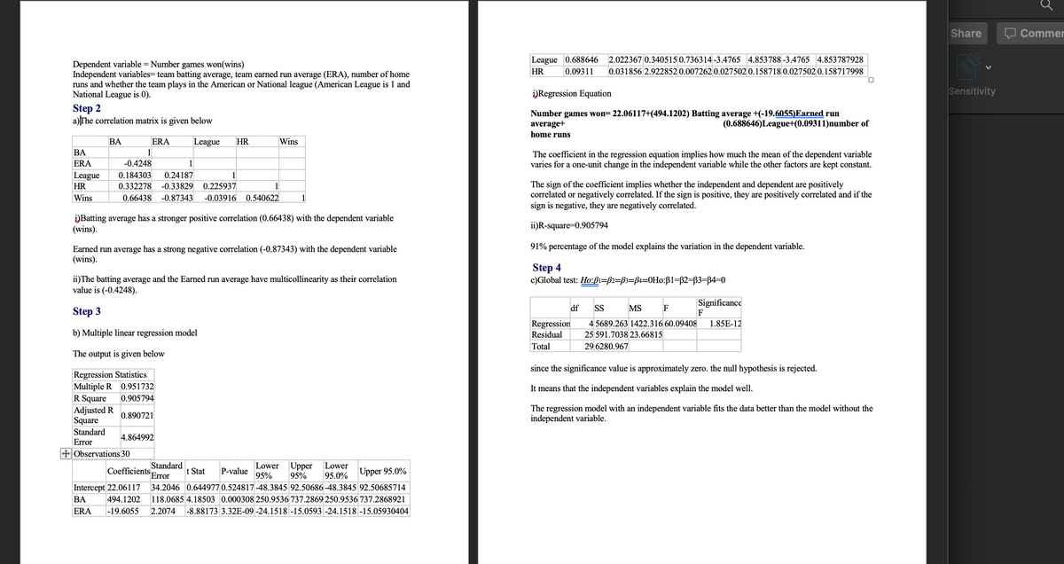
a) The correlation matrix is given below
Number games won= 22.06117+(494.1202) Batting average +(-19.6055)Earned run
average+
home runs
(0.688646)League+(0.09311)number of
ВА
ERA
League
HR
Wins
BА
1
The coefficient in the regression equation implies how much the mean of the dependent variable
varies for a one-unit change in the independent variable while the other factors are kept constant.
ERA
-0.4248
1
League
0.184303
0.24187
The sign of the coefficient implies whether the independent and dependent are positively
correlated or negatively correlated. If the sign is positive, they are positively correlated and if the
sign is negative, they are negatively correlated.
HR
0.332278
-0.33829
0.225937
1
Wins
0.66438
-0.87343
-0.03916 0.540622
1
)Batting average has a stronger positive correlation (0.66438) with the dependent variable
(wins).
ii)R-square=0.905794
91% percentage of the model explains the variation in the dependent variable.
Earned run average has a strong negative correlation (-0.87343) with the dependent variable
(wins).
Step 4
c)Global test: Ho:ß1=B2=ß3=B4=0Ho:B1=B2=B3=B4=0
ii)The batting average and the Earned run average have multicollinearity as their correlation
value is (-0.4248).
Significance
F
df
SS
MS
F
Step 3
Regression
Residual
4 5689.263 1422.316 60.09408
1.85E-12
b) Multiple linear regression model
25 591.7038 23.66815
Total
29 6280.967
The output is given below
since the significance value is approximately zero. the null hypothesis is rejected.
Regression Statistics
Multiple R 0.951732
R Square
Adjusted R
Square
Standard
It means that the independent variables explain the model well.
0.905794
The regression model with an independent variable fits the data better than the model without the
independent variable.
0.890721
4.864992
Error
+ Observations 30
Standard
Error
Lower Upper
95%
95%
Lower
Coefficients
t Stat
P-value
Upper 95.0%
95.0%
Intercept 22.06117
34.2046 0.644977 0.52481748.3845 92.50686-48.3845 92.50685714
ВА
494.1202
118.0685 4.18503 0.000308 250.9536 737.2869 250.9536 737.2868921
ERA
-19.6055
2.2074
-8.88173 3.32E-09 -24.1518 -15.0593 -24.1518 -15.05930404
Expert Solution
This question has been solved!
Explore an expertly crafted, step-by-step solution for a thorough understanding of key concepts.

This is a popular solution!

Trending now
This is a popular solution!

Step by step
Solved in 3 steps with 4 images

Knowledge Booster


Learn more about
Need a deep-dive on the concept behind this application? Look no further. Learn more about this topic, statistics and related others by exploring similar questions and additional content below.Recommended textbooks for you
Linear Algebra: A Modern Introduction
Algebra
ISBN:
9781285463247
Author:
David Poole
Publisher:
Cengage Learning

Algebra & Trigonometry with Analytic Geometry
Algebra
ISBN:
9781133382119
Author:
Swokowski
Publisher:
Cengage

Glencoe Algebra 1, Student Edition, 9780079039897…
Algebra
ISBN:
9780079039897
Author:
Carter
Publisher:
McGraw Hill
Linear Algebra: A Modern Introduction
Algebra
ISBN:
9781285463247
Author:
David Poole
Publisher:
Cengage Learning
Algebra & Trigonometry with Analytic Geometry
Algebra
ISBN:
9781133382119
Author:
Swokowski
Publisher:
Cengage
Glencoe Algebra 1, Student Edition, 9780079039897…
Algebra
ISBN:
9780079039897
Author:
Carter
Publisher:
McGraw Hill

Holt Mcdougal Larson Pre-algebra: Student Edition…
Algebra
ISBN:
9780547587776
Author:
HOLT MCDOUGAL
Publisher:
HOLT MCDOUGAL