Suppose X1,..., Xn F with mean µ and variance o². (F is a general (b) distribution and not necessarily normal.) When n is large, show that r (x. 1.96-
Suppose X1,..., Xn F with mean µ and variance o². (F is a general (b) distribution and not necessarily normal.) When n is large, show that r (x. 1.96-

MATLAB: An Introduction with Applications
6th Edition
ISBN:9781119256830
Author:Amos Gilat
Publisher:Amos Gilat
Chapter1: Starting With Matlab
Section: Chapter Questions
Problem 1P

Related questions
Question
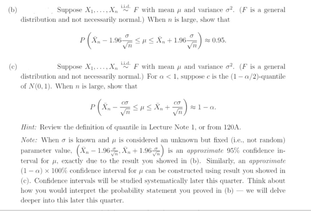
Transcribed Image Text:Suppose X1,..., Xn F with mean µ and variance o². (F is a general
(b)
distribution and not necessarily normal.) When n is large, show that
r(x.
1.96-
<HS Xn + 1.96–
2 0.95.
Suppose X1,..., X,
i.i.d.
* F with mean µ and variance o². (F is a general
(c)
distribution and not necessarily normal.) For a < 1, suppose c is the (1 – a/2)-quantile
of N(0, 1). When n is large, show that
CƠ
CƠ
P ( Xn - SHS Xn +
21– a.
Hint: Review the definition of quantile in Lecture Note 1, or from 120A.
Note: When o is known and µ is considered an unknown but fixed (i.e., not random)
parameter value, (X„ – 1.96-, X„ + 1.96) is an approrimate 95% confidence in-
terval for µ, exactly due to the result you showed in (b). Similarly, an approximate
(1 – a) × 100% confidence interval for µ can be constructed using result you showed in
(c). Confidence intervals will be studied systematically later this quarter. Think about
Vn
how you would interpret the probability statement you proved in (b)
we will delve
deeper into this later this quarter.
Expert Solution
This question has been solved!
Explore an expertly crafted, step-by-step solution for a thorough understanding of key concepts.

Step by step
Solved in 2 steps with 2 images

Recommended textbooks for you
MATLAB: An Introduction with Applications
Statistics
ISBN:
9781119256830
Author:
Amos Gilat
Publisher:
John Wiley & Sons Inc

Probability and Statistics for Engineering and th…
Statistics
ISBN:
9781305251809
Author:
Jay L. Devore
Publisher:
Cengage Learning

Statistics for The Behavioral Sciences (MindTap C…
Statistics
ISBN:
9781305504912
Author:
Frederick J Gravetter, Larry B. Wallnau
Publisher:
Cengage Learning
MATLAB: An Introduction with Applications
Statistics
ISBN:
9781119256830
Author:
Amos Gilat
Publisher:
John Wiley & Sons Inc
Probability and Statistics for Engineering and th…
Statistics
ISBN:
9781305251809
Author:
Jay L. Devore
Publisher:
Cengage Learning
Statistics for The Behavioral Sciences (MindTap C…
Statistics
ISBN:
9781305504912
Author:
Frederick J Gravetter, Larry B. Wallnau
Publisher:
Cengage Learning

Elementary Statistics: Picturing the World (7th E…
Statistics
ISBN:
9780134683416
Author:
Ron Larson, Betsy Farber
Publisher:
PEARSON

The Basic Practice of Statistics
Statistics
ISBN:
9781319042578
Author:
David S. Moore, William I. Notz, Michael A. Fligner
Publisher:
W. H. Freeman

Introduction to the Practice of Statistics
Statistics
ISBN:
9781319013387
Author:
David S. Moore, George P. McCabe, Bruce A. Craig
Publisher:
W. H. Freeman