TABLE 1.2 0.00 0.010.020.03 0.04 0.05 0.06 0.07 0.08 0.09 Z 0.0 0.504 0.508 0.5120.516 0.5199 0.5239 0.5279 0.5319 0.5359 0.0 0.1 0.5398 0.5438 0.5478 0.5517 0.5557 0.5596 0.5636 0.5675 0.5714 0.5753 0.1 0.20.5793 0.5832 0.5871 0.591 0.5948 0.5987 06026 0.6064 0.6103 0.6141 0.2 6179 0.6217 0.6255 0.6293 0.6331 0.6368 0.6406 0.6443 0.648 0.6517 0.3 6554 0.6591 0.6628 0.6664 0.670.6736 0.6772 0.6808 0.6844 0.6879 0.4 0.6915 0.695 0.6985 0.7019 0.7054 0.7088 0.7123 0.7157 0.719 0.7224 0.5 0.6 0.7257 0.7291 0.73240.7357 0.7389 0.7422 0.7454 0.7486 0.7517 0.7549 0.6 0.758 0.7611 0.7642 0.7673 0.7704 0.7734 0.7764 0.7794 0.7823 0.7852 0.7 7881 0.791 0.7939 0.7967 0.7995 0.8023 0.8051 0.8078 0.8106 0.8133 0.8 8159 0.8186 0.8212 0.8238 0.8264 0.8289 0.8315 0.834 0.8365 0.8389 0.9 0.3 0.4 0.8 0.9 TABLE 1.2: (continued) 1.0 | 0.8413| 0.8438| 0.8461| 0.8485| 0.8508| 0.8531| 0.8554| O.857기 0.8599| 0.8621| 1.0 0.8997 0.9015 1.2 14 0.9192 0.9207 0.9222 0.9236 0.9292 0.9306 0.9319 1.4 8643 0.8665 0.8686 0.8708 0.8729 0.8749 0.87 879 0.883 0.8849 0.8869 0.8888 0.8907 0.8925 0.8944 0.89620.8980 0.9032 0.9049 0.90660.90820.9099 9147 0.9251 0.9265 0.9279 2 0.9394 0.94060.9418 0.9429 0.9441 35 0.9545 9573 0.9582 0.9591 0.9599 0.9608 0.9616 0.9625 0.9633 0.9641 0.9649 0.9656 0.9664 0.9671 0.9678 0.9686 0.9693 0.9699 0.9706 61 0.9767 9332 0.9345 0.9357 0.937 0.938 9452 0.9 9554 0.9564 0. 0.9474 0 84 0.9495 9515 0.9525 1.7 9713 0.9 9 0.972 7210 2.1 0.9821 0.9826 0.983 0.9834 0.9838 0.9842 0.9846 0.985 0.9854 0.9857 2.1 0.9878 0.9881 0.9884 0.9887 0.989 2.2 2.3 9929 0.9931 0.9932 0.9934 0.9936 2.4 0.9861 0.9864 0.9868 0.9871 0.9875 2.3 9893 0.9896 0.9898 0.9901 0.9904 0.9906 0.9909 0.9911 0.9913 0.9916 9918 0.992 9953 0.9955 0.9956 0.9957 0.9959 0.996 0.9961 0.9962 0.9963 0.9964 9974 0.9975 0.9976 0.9977 0.9977 0.9978 0.997 9987 0.9987 0.9987 0.9988 0.9988 0.9989 0.9989 0.9989 0.999 0.999 9922 0.9925 0.992 0.994 0.9941 3 0.9 9949 2.6 9971 0.9972 0.9973 0.9974 2.7 2.7 0.9965 0.9966 0.9967 0.9968 0.9969 0.997 0. 9 09979 0.998 0.9981 28 2.9 0.9981 0.9982 0.9982 0.9983 0.9984 0.9984 0.9985 0.9985 0.9986 0.9986 2.9 3.0 3.0 0.9991 0.9991 0.9991 0.9992 0.9992 0.9992 0.9992 0.9 3.2 0.993 0.9993 0.9994 0.9994 0.9994 0.9994 0.9994 0.9995 0.9995 0.9995 3.2 3.3 0.9995 0.9995 0.9995 0.9996 0.9996 0.9996 0.9996 0.9996 0.9996 0.9997 3.3 3.4 0.9997 0.9997 0.9997 0.9997 0.9997 0.9997 0.99970.9997 0.9997 0.9998 3.4 3.6 0.9998 0.9998 0.9999 0.9999 0.9999 0.9999 0.9999 0.9999 0.9999 0 3.6 0.9999 0.9999 0.9999 0.9999 0.9999 0.9999 0.9999 0.9999 0.9999 0.9999 3.7 3.8 3.9 0.999 3.8 0. 9999 0.9999 0.9999 0.9999 0.9999 0.9999 0.9999 0.9999 0.9999 0.9999 3.9 1 000 0.01 0.02 0.04 08 0.09


Continuous Probability Distributions
Probability distributions are of two types, which are continuous probability distributions and discrete probability distributions. A continuous probability distribution contains an infinite number of values. For example, if time is infinite: you could count from 0 to a trillion seconds, billion seconds, so on indefinitely. A discrete probability distribution consists of only a countable set of possible values.
Normal Distribution
Suppose we had to design a bathroom weighing scale, how would we decide what should be the range of the weighing machine? Would we take the highest recorded human weight in history and use that as the upper limit for our weighing scale? This may not be a great idea as the sensitivity of the scale would get reduced if the range is too large. At the same time, if we keep the upper limit too low, it may not be usable for a large percentage of the population!
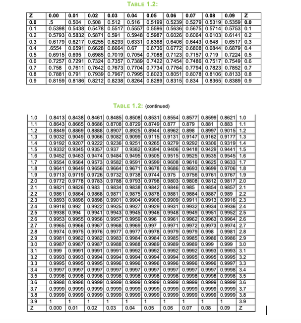
refer to the table attached.
- What is the
probability of the random occurrence of a value between 56 and 61 from anormally distributed population with mean 62 and standard deviation 4.5?


Trending now
This is a popular solution!

Step by step
Solved in 6 steps with 5 images


