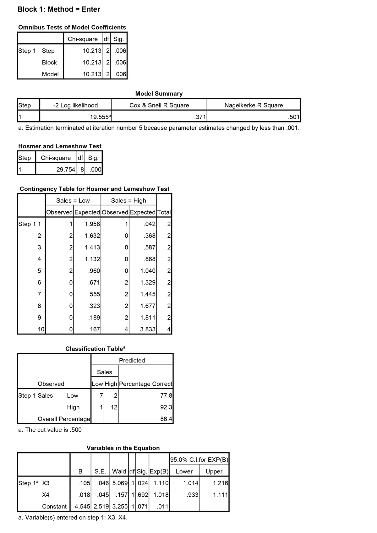
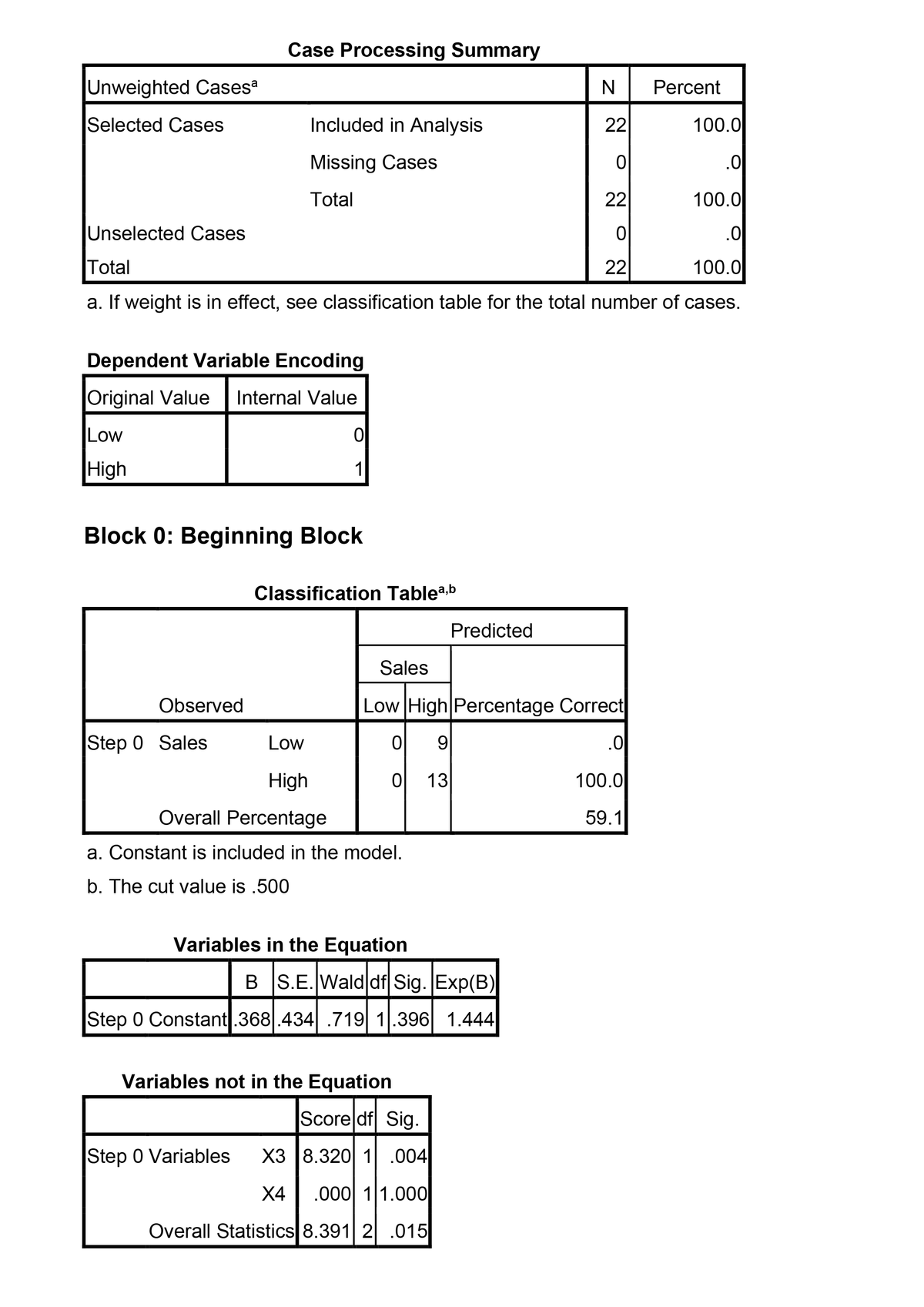
the comic book store owner is curious in how well radio and newspaper advertisements work. A sample of 22 counties with almost equal populations was gathered during the month. For each of the counties, the owner has set aside a particular sum for radio and newspaper advertising. Additionally, the owner was able to access comic book sales information for the stores he controlled in each municipality and classified it as Low or High. COUNTY (X1) Comic book Sales (X2) (0 = Low, 1 = High) Radio Ads (X3) (in thousands) Newspaper Ads (X4) (in thousands) 1 1 0 40 2 0 0 40 3 0 25 25 4 0 25 25 5 0 30 30 6 0 30 30 7 0 35 35 8 0 35 35 9 0 40 25 10 0 40 25 11 1 45 45 12 1 45 45 13 1 50 0 14 1 50 0 15 1 55 25 16 1 55 25 17 1 60 30 18 1 60 30 19 1 65 35 20 1 65 35 21 1 70 40 22 1 70 40 Interpret the Results of the Binary Logistic Regression found in the attached image files


the comic book store owner is curious in how well radio and newspaper advertisements work. A sample of 22 counties with almost equal populations was gathered during the month. For each of the counties, the owner has set aside a particular sum for radio and newspaper advertising. Additionally, the owner was able to access comic book sales information for the stores he controlled in each municipality and classified it as Low or High.
|
COUNTY (X1)
|
Comic book Sales (X2) (0 = Low, 1 = High) |
Radio Ads (X3) (in thousands) |
Newspaper Ads (X4) (in thousands) |
|
1 |
1 |
0 |
40 |
|
2 |
0 |
0 |
40 |
|
3 |
0 |
25 |
25 |
|
4 |
0 |
25 |
25 |
|
5 |
0 |
30 |
30 |
|
6 |
0 |
30 |
30 |
|
7 |
0 |
35 |
35 |
|
8 |
0 |
35 |
35 |
|
9 |
0 |
40 |
25 |
|
10 |
0 |
40 |
25 |
|
11 |
1 |
45 |
45 |
|
12 |
1 |
45 |
45 |
|
13 |
1 |
50 |
0 |
|
14 |
1 |
50 |
0 |
|
15 |
1 |
55 |
25 |
|
16 |
1 |
55 |
25 |
|
17 |
1 |
60 |
30 |
|
18 |
1 |
60 |
30 |
|
19 |
1 |
65 |
35 |
|
20 |
1 |
65 |
35 |
|
21 |
1 |
70 |
40 |
|
22 |
1 |
70 |
40 |
Interpret the Results of the Binary Logistic Regression found in the attached image files

Step by step
Solved in 2 steps with 4 images


