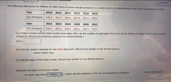
The following table gives the millions of metric tons of carbon dioxide emissions in a certain country for selected years from 2010 and projected to 2032. Year 2010 2012 2014 2016 2018 2020 Co2 Emissions 336.5 362.5 399.1 421.8 451.1 495.4 Year 2022 2024 2026 2028 2030 2032 Co2 Emissions 559.2 591.9 628.7 662.1 701.1 742.7 (a) Create a linear function that models these data, with x as the number of years past 2010 and y as the millions of metric tons of carbon dioxide emissions. (Round all numerical values to two decimal places.) Y(x)- (b) Find the model's estimate for the 2024 data point. (Round your answer to two decimal places.) million metric tons (c) Find the slope of the linear model. (Round your answer to two decimal places.) Interpret the slope of the linear model. million metric tons. carbon dioxide emissions in the U.S. are expected to change by For each year since-Select:


Continuous Probability Distributions
Probability distributions are of two types, which are continuous probability distributions and discrete probability distributions. A continuous probability distribution contains an infinite number of values. For example, if time is infinite: you could count from 0 to a trillion seconds, billion seconds, so on indefinitely. A discrete probability distribution consists of only a countable set of possible values.
Normal Distribution
Suppose we had to design a bathroom weighing scale, how would we decide what should be the range of the weighing machine? Would we take the highest recorded human weight in history and use that as the upper limit for our weighing scale? This may not be a great idea as the sensitivity of the scale would get reduced if the range is too large. At the same time, if we keep the upper limit too low, it may not be usable for a large percentage of the population!


Trending now
This is a popular solution!

Learn your way
Includes step-by-step video

Step by step
Solved in 3 steps with 2 images


