Use the combined data of 80 students, construct a 95% confidence interval estimate of the population proportion of students can pass the aptitude test.

MATLAB: An Introduction with Applications
6th Edition
ISBN:9781119256830
Author:Amos Gilat
Publisher:Amos Gilat
Chapter1: Starting With Matlab
Section: Chapter Questions
Problem 1P
icon
Related questions
Question

PLEASE DO PART D

The education department has conducted a survey to review student’s language ability. A sample of 40 boys and 40 girls have been selected randomly selected for an aptitude test. The test result is that 28 boys pass the test, and 32 girls pass the test.
(a) Give a point estimate of the population proportion of boys can pass the aptitude test.
(b) Give a point estimate of the population proportion of girls can pass the aptitude test.
(c) Use the combined data of 80 students, give a point estimate of the population proportion of students can pass the aptitude test.
(d) Use the combined data of 80 students, construct a 95% confidence interval estimate of the population proportion of students can pass the aptitude test.

The entries in Table I are the probabilities that a random variable having the
standard normal distribution will take on a value between 0 and:. They are given
by the area of the gray region under the curve in the figure.
TABLE I
NORMAL-CURVE AREAS
0.00
0.01
0.02
0.03
0.04
0.05
0.06
0.07
0.08
0.09
0.0
0.0000
0.0040
0.0080
0.0120
0.0160
0.0199
0.0239
0.0279
0.0319
0.0359
0.0398
0.0793
0.0438
0.0832
0.0675
0.1064
0.0517
0.0636
0.1026
0.1
0.0478
0.0557
0.0596
0.0714
0.0753
0.2
0.0871
0.0910
0.0948
0.0987
0.1103
0.1141
0.3
0.1179
0.1217
0.1255
0.1293
0.1331
0.1368
0.1406
0.1443
0.1480
0.1517
0.4
0.1554
0.1591
0.1628
0.1664
0.1700
0.1736
0.1772
0.1808
0.1844
0.1879
0.5
0.1915
0.1950
0.1985
0.2019
0.2054
0.2088
0.2123
0.2157
0.2190
0.2224
0.2257
0.2580
0.2324
0.2642
0.2357
0.2673
0.2389
0.2704
0.2422
0.2734
0.2517
0.2823
0.2549
0.2852
0.6
0.2291
0.2454
0.2486
0.7
0.2611
0.2764
0.2794
0.8
0.3159
0.3413
0.2881
0.2910
0.2939
0.2967
0.2995
0.3023
0.3051
0.3078
0.3106
0.3133
0.9
0.3186
0.3212
0.3238
0.3264
0.3289
0.3315
0.3340
0.3365
0.3389
1.0
0.3438
0.3461
0.3485
0.3508
0.3531
0.3554
0.3577
0.3599
0.3621
0.3686
0.3888
0.4066
0.3770
0.3962
0.4131
1.1
0.3643
0.3665
0.3708
0.3729
0.3749
0.3790
0.3810
0.3830
0.3849
0.4032
0.3907
0.4082
0.4236
0.3997
0.4162
0.4306
0.3869
0.3925
0.4099
0.4251
1.2
0.3944
0.3980
0.4015
0.4049
0.4207
1.3
0.4115
0.4147
0.4177
1.4
0.4192
0.4222
0.4265
0.4279
0.4292
0.4319
1.5
0.4332
0.4345
0.4357
0.4370
0.4382
0.4394
0.4406
0.4418
0.4429
0.4441
0.4484
0.4582
0.4664
0.4535
0.4625
0.4699
1.6
0.4452
0.4463
0.4474
0.4495
0.4505
0.4515
0.4525
0.4545
0.4554
0.4641
0.4564
0.4648
0.4591
0.4671
0.4608
0.4685
0.4616
0.4692
0.4633
0.4706
1.7
0.4573
0.4599
1.8
0.4656
0.4678
1.9
0.4713
0.4719
0.4725
0.4732
0.4738
0.4744
0.4750
0.4756
0.4761
0.4767
2.0
0.4772
0.4778
0.4783
0.4788
0.4793
0.4798
0.4803
0.4808
0.4812
0.4817
0.4821
0.4861
0.4834
0.4871
0.4901
0.4838
0.4875
0.4904
0.4846
0.4881
0.4909
0.4857
0.4890
2.1
0.4826
0.4830
0.4842
0.4850
0.4854
0.4875
0.4906
0.4887
0.4913
2.2
0.4864
0.4868
0.4884
2.3
0.4893
0.4896
0.4898
0.4911
0.4916
2.4
0.4918
0.4920
0.4922
0.4925
0.4927
0.4929
0.4931
0.4932
0.4934
0.4936
2.5
0.4938
0.4940
0.4941
0.4943
0.4945
0.4946
0.4948
0.4949
0.4951
0.4952
0.4957
0.4968
0.4963
0.4973
0.4953
0.4955
0.4966
0.4959
0.4969
2.6
0.4956
0.4960
0.4961
0.4962
0.4964
0.4974
2.7
0.4965
0.4967
0.4970
0.4971
0.4972
2.8
0.4974
0.4975
0.4976
0.4977
0.4977
0.4978
0.4979
0.4979
0.4980
0.4981
2.9
0.4981
0.4982
0.4982
0.4983
0.4984
0.4984
0.4985
0.4985
0.4986
0.4986
3.0
0.4987
0.4987
0.4987
0.4988
0.4988
0.4989
0.4989
0.4989
0.4990
0.4990
Also, for z= 4.0, 5.0 and 6.0, the areas are 0.49997, 0.4999997, and 0.499999999.
Transcribed Image Text:The entries in Table I are the probabilities that a random variable having the standard normal distribution will take on a value between 0 and:. They are given by the area of the gray region under the curve in the figure. TABLE I NORMAL-CURVE AREAS 0.00 0.01 0.02 0.03 0.04 0.05 0.06 0.07 0.08 0.09 0.0 0.0000 0.0040 0.0080 0.0120 0.0160 0.0199 0.0239 0.0279 0.0319 0.0359 0.0398 0.0793 0.0438 0.0832 0.0675 0.1064 0.0517 0.0636 0.1026 0.1 0.0478 0.0557 0.0596 0.0714 0.0753 0.2 0.0871 0.0910 0.0948 0.0987 0.1103 0.1141 0.3 0.1179 0.1217 0.1255 0.1293 0.1331 0.1368 0.1406 0.1443 0.1480 0.1517 0.4 0.1554 0.1591 0.1628 0.1664 0.1700 0.1736 0.1772 0.1808 0.1844 0.1879 0.5 0.1915 0.1950 0.1985 0.2019 0.2054 0.2088 0.2123 0.2157 0.2190 0.2224 0.2257 0.2580 0.2324 0.2642 0.2357 0.2673 0.2389 0.2704 0.2422 0.2734 0.2517 0.2823 0.2549 0.2852 0.6 0.2291 0.2454 0.2486 0.7 0.2611 0.2764 0.2794 0.8 0.3159 0.3413 0.2881 0.2910 0.2939 0.2967 0.2995 0.3023 0.3051 0.3078 0.3106 0.3133 0.9 0.3186 0.3212 0.3238 0.3264 0.3289 0.3315 0.3340 0.3365 0.3389 1.0 0.3438 0.3461 0.3485 0.3508 0.3531 0.3554 0.3577 0.3599 0.3621 0.3686 0.3888 0.4066 0.3770 0.3962 0.4131 1.1 0.3643 0.3665 0.3708 0.3729 0.3749 0.3790 0.3810 0.3830 0.3849 0.4032 0.3907 0.4082 0.4236 0.3997 0.4162 0.4306 0.3869 0.3925 0.4099 0.4251 1.2 0.3944 0.3980 0.4015 0.4049 0.4207 1.3 0.4115 0.4147 0.4177 1.4 0.4192 0.4222 0.4265 0.4279 0.4292 0.4319 1.5 0.4332 0.4345 0.4357 0.4370 0.4382 0.4394 0.4406 0.4418 0.4429 0.4441 0.4484 0.4582 0.4664 0.4535 0.4625 0.4699 1.6 0.4452 0.4463 0.4474 0.4495 0.4505 0.4515 0.4525 0.4545 0.4554 0.4641 0.4564 0.4648 0.4591 0.4671 0.4608 0.4685 0.4616 0.4692 0.4633 0.4706 1.7 0.4573 0.4599 1.8 0.4656 0.4678 1.9 0.4713 0.4719 0.4725 0.4732 0.4738 0.4744 0.4750 0.4756 0.4761 0.4767 2.0 0.4772 0.4778 0.4783 0.4788 0.4793 0.4798 0.4803 0.4808 0.4812 0.4817 0.4821 0.4861 0.4834 0.4871 0.4901 0.4838 0.4875 0.4904 0.4846 0.4881 0.4909 0.4857 0.4890 2.1 0.4826 0.4830 0.4842 0.4850 0.4854 0.4875 0.4906 0.4887 0.4913 2.2 0.4864 0.4868 0.4884 2.3 0.4893 0.4896 0.4898 0.4911 0.4916 2.4 0.4918 0.4920 0.4922 0.4925 0.4927 0.4929 0.4931 0.4932 0.4934 0.4936 2.5 0.4938 0.4940 0.4941 0.4943 0.4945 0.4946 0.4948 0.4949 0.4951 0.4952 0.4957 0.4968 0.4963 0.4973 0.4953 0.4955 0.4966 0.4959 0.4969 2.6 0.4956 0.4960 0.4961 0.4962 0.4964 0.4974 2.7 0.4965 0.4967 0.4970 0.4971 0.4972 2.8 0.4974 0.4975 0.4976 0.4977 0.4977 0.4978 0.4979 0.4979 0.4980 0.4981 2.9 0.4981 0.4982 0.4982 0.4983 0.4984 0.4984 0.4985 0.4985 0.4986 0.4986 3.0 0.4987 0.4987 0.4987 0.4988 0.4988 0.4989 0.4989 0.4989 0.4990 0.4990 Also, for z= 4.0, 5.0 and 6.0, the areas are 0.49997, 0.4999997, and 0.499999999.
The entries in Table II are values for which the area to their right under the
distribution with given degrees of freedom (the gray area in the figuure) is equal
to a .
t
TABLE II
VALUE OFt
d.f.
f0.050
f0.025
fo.010
f0.005
d.f
1
6.314
12.706
31.821
63.657
1
2.920
4.303
6.965
9.925
2.353
3.182
4.541
5.841
4
2.132
2.776
3.747
4.604
4
5
2.015
2.571
3.365
4.032
1.943
2.447
3.143
3.707
6
7
1.895
2.365
2.998
3.499
7
1.860
2.306
2.896
3.355
9
1.833
2.262
2.821
3.250
9
10
1.812
2.228
2.764
3.169
10
11
1.796
2.201
2.718
3.106
11
12
1.782
2.179
2.681
3.055
12
13
1.771
2.160
2.650
3.012
13
14
1.761
2.145
2.624
2.977
14
15
1.753
2.131
2.602
2.947
15
16
1.746
2.120
2.583
2.921
16
17
1.740
2.110
2.567
2.898
17
18
1.734
2.101
2.552
2.878
18
19
1.729
2.093
2.539
2.861
19
20
1.725
2.086
2.528
2.845
20
21
1.721
2.080
2.518
2.831
21
22
1.717
2.074
2.508
2.819
22
23
1.714
2.069
2.500
2.807
23
24
1.711
2.064
2.492
2.797
24
25
1.708
2.060
2485
2.787
25
26
1.706
2.056
2.479
2.779
26
27
1.703
2.052
2.473
2.771
27
28
1.701
2.048
2.467
2.763
28
29
1.699
2.045
2.462
2.756
29
Inf.
1.645
1.960
2.326
2.576
In.
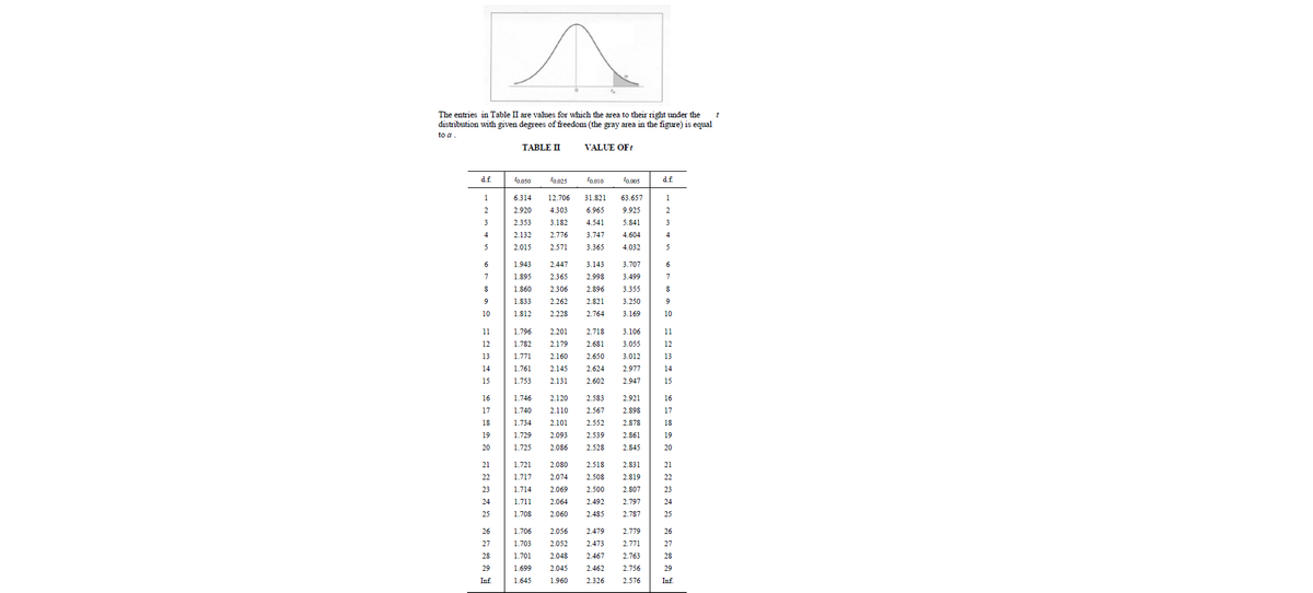
Transcribed Image Text:The entries in Table II are values for which the area to their right under the distribution with given degrees of freedom (the gray area in the figuure) is equal to a . t TABLE II VALUE OFt d.f. f0.050 f0.025 fo.010 f0.005 d.f 1 6.314 12.706 31.821 63.657 1 2.920 4.303 6.965 9.925 2.353 3.182 4.541 5.841 4 2.132 2.776 3.747 4.604 4 5 2.015 2.571 3.365 4.032 1.943 2.447 3.143 3.707 6 7 1.895 2.365 2.998 3.499 7 1.860 2.306 2.896 3.355 9 1.833 2.262 2.821 3.250 9 10 1.812 2.228 2.764 3.169 10 11 1.796 2.201 2.718 3.106 11 12 1.782 2.179 2.681 3.055 12 13 1.771 2.160 2.650 3.012 13 14 1.761 2.145 2.624 2.977 14 15 1.753 2.131 2.602 2.947 15 16 1.746 2.120 2.583 2.921 16 17 1.740 2.110 2.567 2.898 17 18 1.734 2.101 2.552 2.878 18 19 1.729 2.093 2.539 2.861 19 20 1.725 2.086 2.528 2.845 20 21 1.721 2.080 2.518 2.831 21 22 1.717 2.074 2.508 2.819 22 23 1.714 2.069 2.500 2.807 23 24 1.711 2.064 2.492 2.797 24 25 1.708 2.060 2485 2.787 25 26 1.706 2.056 2.479 2.779 26 27 1.703 2.052 2.473 2.771 27 28 1.701 2.048 2.467 2.763 28 29 1.699 2.045 2.462 2.756 29 Inf. 1.645 1.960 2.326 2.576 In.
Expert Solution
steps

Step by step

Solved in 2 steps

Blurred answer
Recommended textbooks for you
MATLAB: An Introduction with Applications
Statistics
ISBN:
9781119256830
Author:
Amos Gilat
Publisher:
John Wiley & Sons Inc
Probability and Statistics for Engineering and th…
Statistics
ISBN:
9781305251809
Author:
Jay L. Devore
Publisher:
Cengage Learning
Statistics for The Behavioral Sciences (MindTap C…
Statistics
ISBN:
9781305504912
Author:
Frederick J Gravetter, Larry B. Wallnau
Publisher:
Cengage Learning
Elementary Statistics: Picturing the World (7th E…
Statistics
ISBN:
9780134683416
Author:
Ron Larson, Betsy Farber
Publisher:
PEARSON
The Basic Practice of Statistics
Statistics
ISBN:
9781319042578
Author:
David S. Moore, William I. Notz, Michael A. Fligner
Publisher:
W. H. Freeman
Introduction to the Practice of Statistics
Statistics
ISBN:
9781319013387
Author:
David S. Moore, George P. McCabe, Bruce A. Craig
Publisher:
W. H. Freeman