a) State the null and alternative hypothesis in this global test for linear model utility. b) Give the p-value and your conclusion. c) Conduct t-tests on each of the beta parameters. What is your conclusion in each case? d) What percentage of the variation in the price is explained by these independent variables? Based on this, is a multiple linear regression model a good model for these data? Explain. e) Give the point estimate for the price of a 44 year old single family home in Beavercreek, OH with 1704 square feet of living space, 3 bedrooms, and 2.5 bathrooms.
a) State the null and alternative hypothesis in this global test for linear model utility. b) Give the p-value and your conclusion. c) Conduct t-tests on each of the beta parameters. What is your conclusion in each case? d) What percentage of the variation in the price is explained by these independent variables? Based on this, is a multiple linear regression model a good model for these data? Explain. e) Give the point estimate for the price of a 44 year old single family home in Beavercreek, OH with 1704 square feet of living space, 3 bedrooms, and 2.5 bathrooms.

Algebra and Trigonometry (MindTap Course List)
4th Edition
ISBN:9781305071742
Author:James Stewart, Lothar Redlin, Saleem Watson
Publisher:James Stewart, Lothar Redlin, Saleem Watson
Chapter1: Equations And Graphs
Section1.FOM: Focus On Modeling: Fitting Lines To Data
Problem 7P

Related questions
Question
d and c
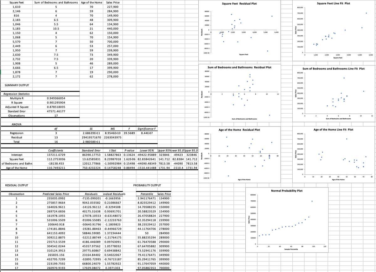
Transcribed Image Text:Square Feet
Sum of Bedrooms and Bathrooms Age of the Home
Sales Price
Square Feet Residual Plot
Square Feet Line Fit Plot
1,610
5
70
227,900
800,000
2,146
6
59
284,900
700,000
816
4
70
149,900
FO000
600,000
2,183
6.5
48
309,900
40000
1,046
5.5
64
134,900
500.000
20000
5,183
10.5
21
440,000
400,000
• 2 000
1,150
4
62
150,000
1,000
4,000
5.000
6,000
2000 0
300,000
1,068
70
154,900
4000 0
5,570
7
50
700,000
200,000
6000 0
2,449
6.
53
257,000
100,000
BO00 0
1,950
59
239,900
1000 00
2,630
7.5
73
349,900
Square Feet
1,000
2,000
3,000
4,000
5,000
6,000
Square Feet
2,732
7.5
20
339,900
1,908
5
46
289,000
3,666
6.5
17
399,900
Sum of Bedrooms and Bathrooms Residual Plot
Sum of Bedrooms and Bathrooms Line Fit Plot
80000
1,878
7
19
290,000
800,000
2,172
62
278,000
60000
700,000
40000
600,000
SUMMARY OUTPUT
20000
500,000
400,000
Regression Statistics
12
2000 0
Multiple R
0.949366054
300,000
R Square
0.901295904
4000 0
200,000
Adjusted R Square
0.878518035
6000 0
100,000
Standard Error
47571.46177
8000 0
Observations
17
2
12
1000 00
Sum of Bedrooms and Bathrooms
Sum of Bedrooms and Bathrooms
ANOVA
df
SS
MS
F
Significance F
Age of the Home Residual Plot
Age of the Home Line Fit Plot
Regression
3
2.68639E+11
8.9546E+10 39.5689
8,44E-07
80000
800,000
Residual
13
29419571670 2263043975
60000
700,000
Total
16
2.98058E+11
40000
20000
500,000
t Stat
1.588278630.13624 -49422.95889 323846
Coefficients
Standard Error
P-value
Lower 95% Upper 95%ɔwer 95.0spper 95.0
-49423
323846
400,000
Intercept
137211.6729
86390,17753
10
20
60
80
Square Feet
13.62585831
2000 0
112.2753036
8.23987018 1.62E-06 82.83842641 141.712 82.8384 141.712
300,000
of Bedrooms and Bathro
-18138.453
12012.77866
-1.50992984 0.15498 -44090.48349 7813.58
-44090
7813,58
4000 0
200,000
Age of the Home
110.7493211
750.4232224
0.14758248
0.88494 -1510.441488 1731.94
-1510.4 1731.94
100,000
8000 0
80
1000 00
Age of the Home
Age of the Home
RESIDUAL OUTPUT
PROBABILITY OUTPUT
Normal Probability Plot
Observation
Predicted Sales Price
Residuals
indard Residuals
Percentile
Sales Price
800000
235035.0992
-7135.099201
-0.1663956
2,941176471 134900
700000
275857.9664
9042.033582
0.21086667
8.823529412
149900
3
164026.9611
-14126.96112
-0.3294508
14.70588235
150000
4
269724.6836
40175.31638
0.93691701
20.58823529
154900
So000
5
161978.1055
-27078.10553
-0.63148072
26.47058824
227900
531006.5509
-91006.55085 -2.12233763
32.35294118
239900
* 400000
7
200640.918
-50640.91796
-1.1809823
38.23529412
257000
300000
8
174181.8846
-19281.88463 -0.44966729
44.11764706 278000
200000
641153.4092
58846.59085
1.37234444
50
284900
10
309212.8875
-52212.88749
-1.21764175
55.88235294
289000
100000
11
235713.5539
4186.446089
0.09763091
61.76470588
290000
12
304542.0244
45357.97562
1.05778032
67.64705882
309900
20
40
60
80
100
120
Sample Percentile
13
310124.3913
29775.60867
0.69438842
73.52941176
339900
14
265835.156
23164.84402
0.54022067
79.41176471
349900
15
432795.7299
-32895.72995
-0.76715187
85.29411765
399900
16
223199.7592
66800.24079
1.55782922
91.17647059
440000
17
260970.9193
17029.08072
0.3971303
97.05882353
700000
Transcribed Image Text:a) State the null and alternative hypothesis in this global test for linear model utility.
b) Give the p-value and your conclusion.
c) Conduct t-tests on each of the beta parameters. What is your conclusion in each case?
d) What percentage of the variation in the price is explained by these independent variables?
Based on this, is a multiple linear regression model a good model for these data? Explain.
e) Give the point estimate for the price of a 44 year old single family home in Beavercreek, OH
with 1704 square feet of living space, 3 bedrooms, and 2.5 bathrooms.
Expert Solution
This question has been solved!
Explore an expertly crafted, step-by-step solution for a thorough understanding of key concepts.

Step by step
Solved in 2 steps with 2 images

Recommended textbooks for you
Algebra and Trigonometry (MindTap Course List)
Algebra
ISBN:
9781305071742
Author:
James Stewart, Lothar Redlin, Saleem Watson
Publisher:
Cengage Learning

Algebra & Trigonometry with Analytic Geometry
Algebra
ISBN:
9781133382119
Author:
Swokowski
Publisher:
Cengage

Linear Algebra: A Modern Introduction
Algebra
ISBN:
9781285463247
Author:
David Poole
Publisher:
Cengage Learning
Algebra and Trigonometry (MindTap Course List)
Algebra
ISBN:
9781305071742
Author:
James Stewart, Lothar Redlin, Saleem Watson
Publisher:
Cengage Learning
Algebra & Trigonometry with Analytic Geometry
Algebra
ISBN:
9781133382119
Author:
Swokowski
Publisher:
Cengage
Linear Algebra: A Modern Introduction
Algebra
ISBN:
9781285463247
Author:
David Poole
Publisher:
Cengage Learning

Functions and Change: A Modeling Approach to Coll…
Algebra
ISBN:
9781337111348
Author:
Bruce Crauder, Benny Evans, Alan Noell
Publisher:
Cengage Learning

Glencoe Algebra 1, Student Edition, 9780079039897…
Algebra
ISBN:
9780079039897
Author:
Carter
Publisher:
McGraw Hill

College Algebra
Algebra
ISBN:
9781305115545
Author:
James Stewart, Lothar Redlin, Saleem Watson
Publisher:
Cengage Learning