B. Analyze and solve the following problem. The researcher wants to determine wheter the mean lifespan of his specimen of 28 in number is significantly different from the average lifespan of the population which is 95 days. The mean and standard deviation of the lifespan of his specimen is 90 days and 10 days, respectively. Assume a 90% confidence level and interpret the result.
B. Analyze and solve the following problem. The researcher wants to determine wheter the mean lifespan of his specimen of 28 in number is significantly different from the average lifespan of the population which is 95 days. The mean and standard deviation of the lifespan of his specimen is 90 days and 10 days, respectively. Assume a 90% confidence level and interpret the result.

MATLAB: An Introduction with Applications
6th Edition
ISBN:9781119256830
Author:Amos Gilat
Publisher:Amos Gilat
Chapter1: Starting With Matlab
Section: Chapter Questions
Problem 1P

Related questions
Question
Please refer to the lesson and answer the given question
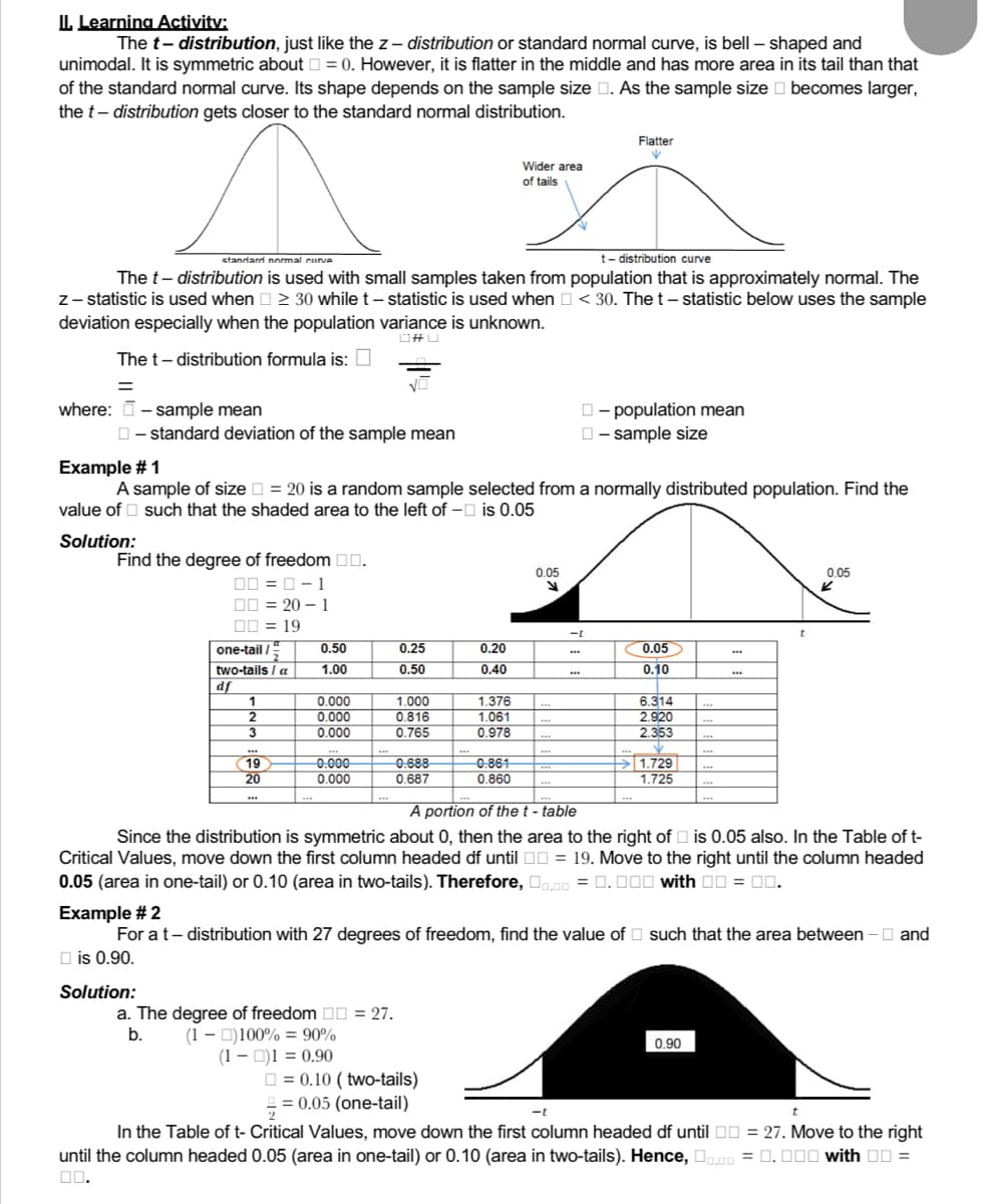
Transcribed Image Text:II. Learning Activity:
The t-distribution, just like the z-distribution or standard normal curve, is bell-shaped and
unimodal. It is symmetric about = 0. However, it is flatter in the middle and has more area in its tail than that
of the standard normal curve. Its shape depends on the sample size . As the sample size becomes larger,
the t - distribution gets closer to the standard normal distribution.
Flatter
V
Wider area
of tails
standardi normal curve
t-distribution curve
The t-distribution is used with small samples taken from population that is approximately normal. The
z - statistic is used when ≥ 30 while t - statistic is used when <30. The t - statistic below uses the sample
deviation especially when the population variance is unknown.
#U
The t - distribution formula is:
=
where: - sample mean
-population mean
- sample size
- standard deviation of the sample mean
Example # 1
A sample of size = 20 is a random sample selected from a normally distributed population. Find the
value of such that the shaded area to the left of - is 0.05
Solution:
Find the degree of freedom 0.
0.05
0.05
y
one-tail/=
0.50
0.25
0.20
0.05
two-tails / a
1.00
0.50
0.40
0.10
df
1
0.000
1.000
1.376
6.314
2
0.000
0.816
1.061
2.920
3
0.000
0.765
0.978
2.353
***
www
19
0.000
0.688
0.861
1.729
20
0.000
0.687
0.860
1.725
A portion of the t - table
Since the distribution is symmetric about 0, then the area to the right of is 0.05 also. In the Table of t-
Critical Values, move down the first column headed df until = 19. Move to the right until the column headed
0.05 (area in one-tail) or 0.10 (area in two-tails). Therefore, D.=0.000 with 00 = 00.
Example # 2
For a t-distribution with 27 degrees of freedom, find the value of such that the area between - and
is 0.90.
Solution:
a. The degree of freedom = 27.
b.
(1)100% = 90%
(1)1 = 0.90
0.90
= 0.10 (two-tails)
== 0.05 (one-tail)
-t
t
In the Table of t-Critical Values, move down the first column headed df until = 27. Move to the right
until the column headed 0.05 (area in one-tail) or 0.10 (area in two-tails). Hence, D.00 = 0.000 with DD =
00.
1-0 =00
00=20-1
□□ = 19
NO
-t
t
Transcribed Image Text:B. Analyze and solve the following problem.
The researcher wants to determine wheter the mean lifespan of his specimen of 28 in number is
significantly different from the average lifespan of the population which is 95 days. The mean and
standard deviation of the lifespan of his specimen is 90 days and 10 days, respectively. Assume a 90%
confidence level and interpret the result.
Expert Solution
This question has been solved!
Explore an expertly crafted, step-by-step solution for a thorough understanding of key concepts.

Step by step
Solved in 2 steps with 1 images

Recommended textbooks for you
MATLAB: An Introduction with Applications
Statistics
ISBN:
9781119256830
Author:
Amos Gilat
Publisher:
John Wiley & Sons Inc

Probability and Statistics for Engineering and th…
Statistics
ISBN:
9781305251809
Author:
Jay L. Devore
Publisher:
Cengage Learning

Statistics for The Behavioral Sciences (MindTap C…
Statistics
ISBN:
9781305504912
Author:
Frederick J Gravetter, Larry B. Wallnau
Publisher:
Cengage Learning
MATLAB: An Introduction with Applications
Statistics
ISBN:
9781119256830
Author:
Amos Gilat
Publisher:
John Wiley & Sons Inc
Probability and Statistics for Engineering and th…
Statistics
ISBN:
9781305251809
Author:
Jay L. Devore
Publisher:
Cengage Learning
Statistics for The Behavioral Sciences (MindTap C…
Statistics
ISBN:
9781305504912
Author:
Frederick J Gravetter, Larry B. Wallnau
Publisher:
Cengage Learning

Elementary Statistics: Picturing the World (7th E…
Statistics
ISBN:
9780134683416
Author:
Ron Larson, Betsy Farber
Publisher:
PEARSON

The Basic Practice of Statistics
Statistics
ISBN:
9781319042578
Author:
David S. Moore, William I. Notz, Michael A. Fligner
Publisher:
W. H. Freeman

Introduction to the Practice of Statistics
Statistics
ISBN:
9781319013387
Author:
David S. Moore, George P. McCabe, Bruce A. Craig
Publisher:
W. H. Freeman