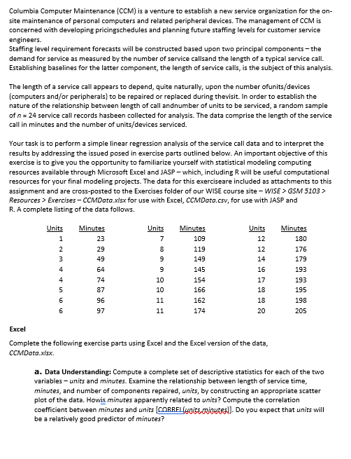
Columbia Computer Maintenance (CCM) is a venture to establish a new service organization for the on- site maintenance of personal computers and related peripheral devices. The management of CCM is concerned with developing pricingschedules and planning future staffing levels for customer service engineers. Staffing level requirement forecasts will be constructed based upon two principal components - the demand for service as measured by the number of service callsand the length of a typical service call. Establishing baselines for the latter component, the length of service calls, is the subject of this analysis. The length of a service call appears to depend, quite naturally, upon the number ofunits/devices (computers and/or peripherals) to be repaired or replaced during thevisit. In order to establish the nature of the relationship between length of call andnumber of units to be serviced, a random sample of n = 24 service call records hasbeen collected for analysis. The data comprise the length of the service call in minutes and the number of units/devices serviced. Your task is to perform a simple linear regression analysis of the service call data and to interpret the results by addressing the issued posed in exercise parts outlined below. An important objective of this exercise is to give you the opportunity to familiarize yourself with statistical modeling computing resources available through Microsoft Excel and JASP - which, including R will be useful computational resources for your final modeling projects. The data for this exerciseare included as attachments to this assignment and are cross-posted to the Exercises folder of our WISE course site-WISE > GSM 5103 > Resources > Exercises - CCMData.xlsx for use with Excel, CCMData.csv, for use with JASP and R. A complete listing of the data follows. Units 1 2 3 4 4 5 6 6 Minutes 23 29 49 $26 25 64 74 87 96 97 Units 7 8 9 9 10 10 11 11 Minutes 109 119 149 145 154 166 162 174 Units 12 12 14 16 17 18 18 20 Excel Complete the following exercise parts using Excel and the Excel version of the data, CCMData.xlsx. Minutes 180 176 179 193 193 195 198 205 a. Data Understanding: Compute a complete set of descriptive statistics for each of the two variables - units and minutes. Examine the relationship between length of service time, minutes, and number of components repaired, units, by constructing an appropriate scatter plot of the data. Howis minutes apparently related to units? Compute the correlation coefficient between minutes and units [CORREL (units minutes)]. Do you expect that units will be a relatively good predictor of minutes?
Columbia Computer Maintenance (CCM) is a venture to establish a new service organization for the on- site maintenance of personal computers and related peripheral devices. The management of CCM is concerned with developing pricingschedules and planning future staffing levels for customer service engineers. Staffing level requirement forecasts will be constructed based upon two principal components - the demand for service as measured by the number of service callsand the length of a typical service call. Establishing baselines for the latter component, the length of service calls, is the subject of this analysis. The length of a service call appears to depend, quite naturally, upon the number ofunits/devices (computers and/or peripherals) to be repaired or replaced during thevisit. In order to establish the nature of the relationship between length of call andnumber of units to be serviced, a random sample of n = 24 service call records hasbeen collected for analysis. The data comprise the length of the service call in minutes and the number of units/devices serviced. Your task is to perform a simple linear regression analysis of the service call data and to interpret the results by addressing the issued posed in exercise parts outlined below. An important objective of this exercise is to give you the opportunity to familiarize yourself with statistical modeling computing resources available through Microsoft Excel and JASP - which, including R will be useful computational resources for your final modeling projects. The data for this exerciseare included as attachments to this assignment and are cross-posted to the Exercises folder of our WISE course site-WISE > GSM 5103 > Resources > Exercises - CCMData.xlsx for use with Excel, CCMData.csv, for use with JASP and R. A complete listing of the data follows. Units 1 2 3 4 4 5 6 6 Minutes 23 29 49 $26 25 64 74 87 96 97 Units 7 8 9 9 10 10 11 11 Minutes 109 119 149 145 154 166 162 174 Units 12 12 14 16 17 18 18 20 Excel Complete the following exercise parts using Excel and the Excel version of the data, CCMData.xlsx. Minutes 180 176 179 193 193 195 198 205 a. Data Understanding: Compute a complete set of descriptive statistics for each of the two variables - units and minutes. Examine the relationship between length of service time, minutes, and number of components repaired, units, by constructing an appropriate scatter plot of the data. Howis minutes apparently related to units? Compute the correlation coefficient between minutes and units [CORREL (units minutes)]. Do you expect that units will be a relatively good predictor of minutes?

MATLAB: An Introduction with Applications
6th Edition
ISBN:9781119256830
Author:Amos Gilat
Publisher:Amos Gilat
Chapter1: Starting With Matlab
Section: Chapter Questions
Problem 1P

Related questions
Question
100%
| Units | Minutes |
| 1 | 23 |
| 2 | 29 |
| 3 | 49 |
| 4 | 64 |
| 4 | 74 |
| 5 | 87 |
| 6 | 96 |
| 6 | 97 |
| 7 | 109 |
| 8 | 119 |
| 9 | 149 |
| 9 | 145 |
| 10 | 154 |
| 10 | 166 |
| 11 | 162 |
| 11 | 174 |
| 12 | 180 |
| 12 | 176 |
| 14 | 179 |
| 16 | 193 |
| 17 | 193 |
| 18 | 195 |
| 18 | 198 |
| 20 | 205 |
CCM DATA
Transcribed Image Text:Columbia Computer Maintenance (CCM) is a venture to establish a new service organization for the on-
site maintenance of personal computers and related peripheral devices. The management of CCM is
concerned with developing pricingschedules and planning future staffing levels for customer service
engineers.
Staffing level requirement forecasts will be constructed based upon two principal components - the
demand for service as measured by the number of service callsand the length of a typical service call.
Establishing baselines for the latter component, the length of service calls, is the subject of this analysis.
The length of a service call appears to depend, quite naturally, upon the number ofunits/devices
(computers and/or peripherals) to be repaired or replaced during thevisit. In order to establish the
nature of the relationship between length of call andnumber of units to be serviced, a random sample
of n = 24 service call records hasbeen collected for analysis. The data comprise the length of the service
call in minutes and the number of units/devices serviced.
Your task is to perform a simple linear regression analysis of the service call data and to interpret the
results by addressing the issued posed in exercise parts outlined below. An important objective of this
exercise is to give you the opportunity to familiarize yourself with statistical modeling computing
resources available through Microsoft Excel and JASP - which, including R will be useful computational
resources for your final modeling projects. The data for this exerciseare included as attachments to this
assignment and are cross-posted to the Exercises folder of our WISE course site-WISE > GSM 5103 >
Resources > Exercises - CCMData.xlsx for use with Excel, CCMDato.csv, for use with JASP and
R. A complete listing of the data follows.
Units
1
2
3
4
4
5
6
6
Minutes
23
29
49
64
74
87
96
97
Units
7
9
9
10
10
11
11
Minutes
109
119
149
145
154
166
162
174
Units
12
12
14
16
17
18
18
20
Excel
Complete the following exercise parts using Excel and the Excel version of the data,
CCMData.xlsx.
Minutes
180
176
179
193
193
195
198
205
a. Data Understanding: Compute a complete set of descriptive statistics for each of the two
variables - units and minutes. Examine the relationship between length of service time,
minutes, and number of components repaired, units, by constructing an appropriate scatter
plot of the data. Howis minutes apparently related to units? Compute the correlation
coefficient between minutes and units [CORREL(ynite, minutes)). Do you expect that units will
be a relatively good predictor of minutes?
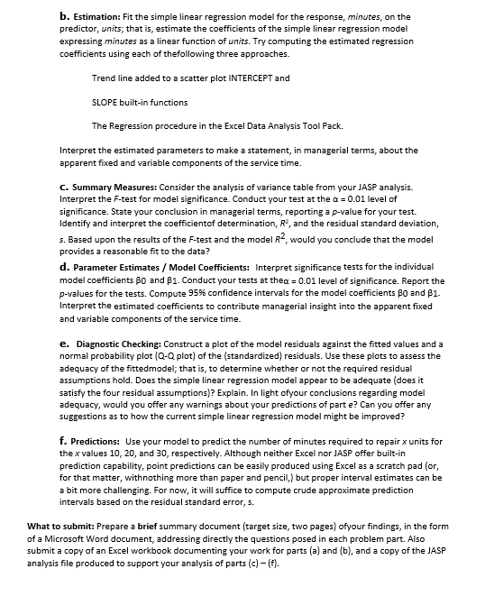
Transcribed Image Text:b. Estimation: Fit the simple linear regression model for the response, minutes, on the
predictor, units; that is, estimate the coefficients of the simple linear regression model
expressing minutes as a linear function of units. Try computing the estimated regression
coefficients using each of the following three approaches.
Trend line added to a scatter plot INTERCEPT and
SLOPE built-in functions
The Regression procedure in the Excel Data Analysis Tool Pack.
Interpret the estimated parameters to make a statement, in managerial terms, about the
apparent fixed and variable components of the service time.
C. Summary Measures: Consider the analysis of variance table from your JASP analysis.
Interpret the F-test for model significance. Conduct your test at the a = 0.01 level of
significance. State your conclusion in managerial terms, reporting a p-value for your test.
Identify and interpret the coefficientof determination, R², and the residual standard deviation,
s. Based upon the results of the F-test and the model R2, would you conclude that the model
provides a reasonable fit to the data?
d. Parameter Estimates / Model Coefficients: Interpret significance tests for the individual
model coefficients 30 and 31. Conduct your tests at thea = 0.01 level of significance. Report the
p-values for the tests. Compute 95% confidence intervals for the model coefficients 30 and 31.
Interpret the estimated coefficients to contribute managerial insight into the apparent fixed
and variable components of the service time.
e. Diagnostic Checking: Construct a plot of the model residuals against the fitted values and a
normal probability plot (Q-Q plot) of the (standardized) residuals. Use these plots to assess the
adequacy of the fittedmodel; that is, to determine whether or not the required residual
assumptions hold. Does the simple linear regression model appear to be adequate (does it
satisfy the four residual assumptions)? Explain. In light ofyour conclusions regarding model
adequacy, would you offer any warnings about your predictions of part e? Can you offer any
suggestions as to how the current simple linear regression model might be improved?
f. Predictions: Use your model to predict the number of minutes required to repair x units for
the x values 10, 20, and 30, respectively. Although neither Excel nor JASP offer built-in
prediction capability, point predictions can be easily produced using Excel as a scratch pad (or,
for that matter, with nothing more than paper and pencil,) but proper interval estimates can be
a bit more challenging. For now, it will suffice to compute crude approximate prediction
intervals based on the residual standard error, s.
What to submit: Prepare a brief summary document (target size, two pages) ofyour findings, in the form
of a Microsoft Word document, addressing directly the questions posed in each problem part. Also
submit a copy of an Excel workbook documenting your work for parts (a) and (b), and a copy of the JASP
analysis file produced to support your analysis of parts (c)- (f).
Expert Solution
This question has been solved!
Explore an expertly crafted, step-by-step solution for a thorough understanding of key concepts.

This is a popular solution!

Trending now
This is a popular solution!

Step by step
Solved in 7 steps with 12 images

Recommended textbooks for you
MATLAB: An Introduction with Applications
Statistics
ISBN:
9781119256830
Author:
Amos Gilat
Publisher:
John Wiley & Sons Inc

Probability and Statistics for Engineering and th…
Statistics
ISBN:
9781305251809
Author:
Jay L. Devore
Publisher:
Cengage Learning

Statistics for The Behavioral Sciences (MindTap C…
Statistics
ISBN:
9781305504912
Author:
Frederick J Gravetter, Larry B. Wallnau
Publisher:
Cengage Learning
MATLAB: An Introduction with Applications
Statistics
ISBN:
9781119256830
Author:
Amos Gilat
Publisher:
John Wiley & Sons Inc
Probability and Statistics for Engineering and th…
Statistics
ISBN:
9781305251809
Author:
Jay L. Devore
Publisher:
Cengage Learning
Statistics for The Behavioral Sciences (MindTap C…
Statistics
ISBN:
9781305504912
Author:
Frederick J Gravetter, Larry B. Wallnau
Publisher:
Cengage Learning

Elementary Statistics: Picturing the World (7th E…
Statistics
ISBN:
9780134683416
Author:
Ron Larson, Betsy Farber
Publisher:
PEARSON

The Basic Practice of Statistics
Statistics
ISBN:
9781319042578
Author:
David S. Moore, William I. Notz, Michael A. Fligner
Publisher:
W. H. Freeman

Introduction to the Practice of Statistics
Statistics
ISBN:
9781319013387
Author:
David S. Moore, George P. McCabe, Bruce A. Craig
Publisher:
W. H. Freeman