Demand Estimation for The San Francisco Bread Company Consider the hypothetical example of The San Francisco Bread Company, a San Francisco-based chain of bakery/cafes. San Francisco Bread Company has initiated an empirical estimation of customer traffic at 30 regional locations to help the firm formulate pricing and promotional plans for the coming year. Annual operating data for the 30 outlets appear in the attached Table 1. The following regression equation was fit to these data: Qi = b0 + b1Pi + b2Pxi + b3Adi + b4Ii + uit. Where: Q is the number of meals served, P is the average price per meal (customer ticket amount, in dollars), Px is the average price charged by competitors (in dollars), Ad is the local advertising budget for each outlet (in dollars), I is the average income per household in each outlet’s service area, ui is a residual (or disturbance) term. The subscript indicates the regional market (i = 1,…, 30) from which the observation was taken. Least squares estimation of the regression equation on the basis of the 30 data cross sectional observations resulted in the estimated regression coefficients and other statistics as shown in Table 2. A. Describe the economic meaning for each individual independent variable included in the San Francisco demand equation. B. Interpret the coefficient of determination (R2) for the San Francisco demand equation. C. What are expected (average) unit sales and sales revenue in a typical market? D. Describe the level statistical significance for each individual independent variable included in the San Francisco demand equation. E. Interpret each coefficient and its impact on the dependent variable. F. Conduct a F-test for the set of coefficients in the equation to determine if they are significant at the 95 and 99 percent levels. (See Below for Data) Table 1 - San Francisco Bread Company (30 Markets) Market Demand Price Competitor Advertising Income Market (Q) (P) Price(Px) (Ad) (I) 1 596,611 7.62 6.52 200,259 54,880 2 596,453 7.29 5.01 204,559 51,755 3 599,201 6.66 5.96 206,647 52,955 4 572,258 8.01 5.30 207,025 54,391 5 558,142 7.53 6.16 207,422 48,491 6 627,973 6.51 7.56 216,224 51,219 7 593,024 6.20 7.15 217,954 48,685 8 565,004 7.28 6.97 220,139 47,219 9 596,254 5.96 5.52 220,215 49,755 10 652,880 6.42 6.27 220,728 54,932 11 596,784 5.94 5.66 226,603 48,092 12 657,468 6.47 7.68 228,620 54,929 13 519,886 6.99 5.10 230,241 46,057 14 612,941 7.72 5.38 232,777 55,239 15 621,707 6.46 6.20 237,300 53,976 16 597,215 7.31 7.43 238,756 49,576 17 617,427 7.36 5.28 241,957 55,454 18 572,320 6.19 6.12 251,317 48,480 19 602,400 7.95 6.38 254,393 53,249 20 575,004 6.34 5.67 255,699 49,696 21 667,581 5.54 7.08 262,270 52,600 22 569,880 7.89 5.10 275,588 50,472 23 644,684 6.76 7.22 277,667 53,409 24 605,468 6.39 5.21 277,816 52,660 25 599,213 6.42 6.00 279,031 50,464 26 610,735 6.82 6.97 279,934 49,525 27 603,830 7.10 5.30 287,921 49,489 28 617,803 7.77 6.96 289,358 49,375 29 529,009 8.07 5.76 294,787 48,254 30 573,211 6.91 5.96 296,246 46,017 Mean 598,412 6.93 6.16 244,649 51,044


Consider the hypothetical example of The San Francisco Bread Company, a San Francisco-based chain of bakery/cafes. San Francisco Bread Company has initiated an empirical estimation of customer traffic at 30 regional locations to help the firm formulate pricing and promotional plans for the coming year. Annual operating data for the 30 outlets appear in the attached Table 1.
The following regression equation was fit to these data:
Qi = b0 + b1Pi + b2Pxi + b3Adi + b4Ii + uit.
Where: Q is the number of meals served,
P is the average price per meal (customer ticket amount, in dollars),
Px is the average price charged by competitors (in dollars),
Ad is the local advertising budget for each outlet (in dollars),
I is the average income per household in each outlet’s service area,
ui is a residual (or disturbance) term.
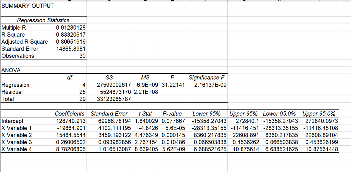
The subscript indicates the regional market (i = 1,…, 30) from which the observation was taken. Least squares estimation of the regression equation on the basis of the 30 data cross sectional observations resulted in the estimated regression coefficients and other statistics as shown in Table 2.
A. Describe the economic meaning for each individual independent variable included in the San Francisco demand equation.
B. Interpret the coefficient of determination (R2) for the San Francisco demand equation.
C. What are expected (average) unit sales and sales revenue in a typical market?
D. Describe the level statistical significance for each individual independent variable included in the San Francisco demand equation.
E. Interpret each coefficient and its impact on the dependent variable.
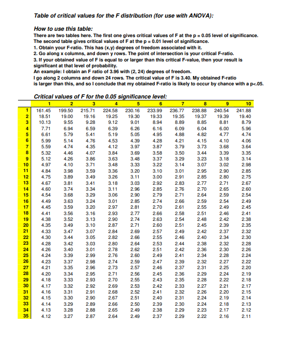
F. Conduct a F-test for the set of coefficients in the equation to determine if they are significant at the 95 and 99 percent levels.
(See Below for Data)
Table 1 - San Francisco Bread Company (30 Markets)
Market Demand Price Competitor Advertising Income
Market (Q) (P) Price(Px) (Ad) (I)
1 596,611 7.62 6.52 200,259 54,880
2 596,453 7.29 5.01 204,559 51,755
3 599,201 6.66 5.96 206,647 52,955
4 572,258 8.01 5.30 207,025 54,391
5 558,142 7.53 6.16 207,422 48,491
6 627,973 6.51 7.56 216,224 51,219
7 593,024 6.20 7.15 217,954 48,685
8 565,004 7.28 6.97 220,139 47,219
9 596,254 5.96 5.52 220,215 49,755
10 652,880 6.42 6.27 220,728 54,932
11 596,784 5.94 5.66 226,603 48,092
12 657,468 6.47 7.68 228,620 54,929
13 519,886 6.99 5.10 230,241 46,057
14 612,941 7.72 5.38 232,777 55,239
15 621,707 6.46 6.20 237,300 53,976
16 597,215 7.31 7.43 238,756 49,576
17 617,427 7.36 5.28 241,957 55,454
18 572,320 6.19 6.12 251,317 48,480
19 602,400 7.95 6.38 254,393 53,249
20 575,004 6.34 5.67 255,699 49,696
21 667,581 5.54 7.08 262,270 52,600
22 569,880 7.89 5.10 275,588 50,472
23 644,684 6.76 7.22 277,667 53,409
24 605,468 6.39 5.21 277,816 52,660
25 599,213 6.42 6.00 279,031 50,464
26 610,735 6.82 6.97 279,934 49,525
27 603,830 7.10 5.30 287,921 49,489
28 617,803 7.77 6.96 289,358 49,375
29 529,009 8.07 5.76 294,787 48,254
30 573,211 6.91 5.96 296,246 46,017
Mean 598,412 6.93 6.16 244,649 51,044


Trending now
This is a popular solution!

Step by step
Solved in 3 steps


