2. Suppose you are to choose among two suppliers of a certain chemical solution used in paint production. The production process yields the best results if the solution has 12% concentration. Both suppliers are capable of producing the desired concentration, however there is naturally occurring random fluc- tuations in the end product. Your analysis of sales samples provided concludes that the solution concentration from Supplier 1 follows a distribution with the density function fi(r) = for 0 < a < 24, whereas the solution concentration from Supplier 2 follows distribution with the probability density function f2(x) = for 0
2. Suppose you are to choose among two suppliers of a certain chemical solution used in paint production. The production process yields the best results if the solution has 12% concentration. Both suppliers are capable of producing the desired concentration, however there is naturally occurring random fluc- tuations in the end product. Your analysis of sales samples provided concludes that the solution concentration from Supplier 1 follows a distribution with the density function fi(r) = for 0 < a < 24, whereas the solution concentration from Supplier 2 follows distribution with the probability density function f2(x) = for 0

MATLAB: An Introduction with Applications
6th Edition
ISBN:9781119256830
Author:Amos Gilat
Publisher:Amos Gilat
Chapter1: Starting With Matlab
Section: Chapter Questions
Problem 1P

Related questions
Question
Please show all your work attached is formula sheet
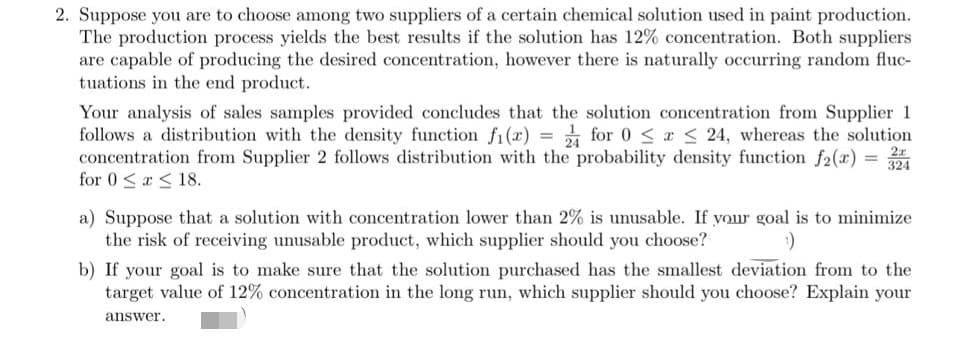
Transcribed Image Text:2. Suppose you are to choose among two suppliers of a certain chemical solution used in paint production.
The production process yields the best results if the solution has 12% concentration. Both suppliers
are capable of producing the desired concentration, however there is naturally occurring random fluc-
tuations in the end product.
Your analysis of sales samples provided concludes that the solution concentration from Supplier 1
follows a distribution with the density function fi(x) = for 0 < a < 24, whereas the solution
2x
324
concentration from Supplier 2 follows distribution with the probability density function f2(x) =
for 0 <a < 18.
a) Suppose that a solution with concentration lower than 2% is unusable. If your goal is to minimize
the risk of receiving unusable product, which supplier should you choose?
b) If your goal is to make sure that the solution purchased has the smallest deviation from to the
target value of 12% concentration in the long run, which supplier should you choose? Explain your
answer.
![Axloms of Probablity
Also Note
1. P(8)-1
2. For any event E, 0S P(E)s1
For any two events A and B,
P(A) - P(AN B) + P(ANB)
3. For any two mutually exclusive events,
and
P(EUF) - P(E) + P(F)
P(AN B) - P(A|B)P(B).
Addition Rule
Events A and B are Independent if:
P(EUF) = P(E) + P(F) - P(En F)
P(A|B) = P(A)
Conditional Probablity
or
P(B|A) -
P(ANB) - P(A)P(B).
PLAN)
Bayes' Theorem:
Total Probablity Rule
P(A|B)P(B)
P(B|A) = PLALBPB) + P(AB)P(B")
P(A) - P(A|B)P(B) + P(A|B')P(B')
Similarly,
Similarly,
P(A) -P(A|E,)P(E)) + P(A|E)P(E)+
...+ P(A|E)P(E)
P(B|E)P(E)
P(E|B) - PIBIE PE) + P(BE PE)+...+ P(B\E)P(E.)
Probability Mass and Density Functions
If X is a discrete r.v:
Cumulative Distribution Function
• F(z) = P(X sz)
P(X = 2) = f(z)
• lim,- F() -0
Es(2) =1 (total probability)
• lim,e F(z) = 1
If X is a continuous r.v.:
P(X = z) = 0
• F(z) = " /(v)dy if X is a contimuous r.v.
S(2)dz =1 (total probability)
• F(z) = E,sz f(z) if X is a discrete r.v.
• P(a < X Sb) - F(b) – F(a)
Expected Value and Variance
Expected Value of a Function of a RV
• E[X) = E, z/(z) if X is a discrete r.v.
• E[h(X)] =E. h(x)f(x) if X is a discrete r.v.
• Eh(X)) = h(z)/(z)dz if X is a continu-
• E[X] = z/(z)dr if X is a continuous r.v.
ous r.v.
• Var(X) = E[Xx] – E[X]?
• E(aX + 6) = aEX] + 6
• Var(aX + b) = a?Var(X)
%3D
• Var(X) = E[(X - E[X])?]
Derivatives and Integrals of Common Functions
• = aea
de
• Sea" dz =
• Sre*dr = e"I- fe*dz = ze" - e (using integration by parts)
dinz
• S !dz = In(z)
Common Discrete Distributions
• X - Bernoulli(p),
if z = 1;
f(z) =
|1-p ifz 0' EX] = p, Var(X) = p(1 – p).
• X- Geometric(p),
f(2) = (1– p)--'p, z E {1,2,..}, E[X] = }, Var(X) = .
Geometric Series: Eg = , for 0 < q < 1
• X - Binomial(n, p),
f(z) = (E) (1– p)"-p*, I € {0, 1,.., n},
E[X] = np, Var(X) = mp(1 – p).
%3D
• X- Negative Binomial(r, p),
f(z) = ()(1 – p)*-"p", E[X] = ;, 1 € {r,r+1,..}, Var(X) = p),
%3D
• X - Hypergeometric(n, M, N),
f(z) =
,
E[X] = n, Var(X) = N=n(1-).
%3D
• X ~ Poisson(At),
f(z) = A0", z e {0, 1, .}, E[X] = At, Var(X) = At.
Common Continuous Distributions
• X - Exponential(A),
f(z) = de-A, z E [0, 00) E[X] = }, Var(X)= .
• X- Erlang(r, A),
f(z) = A' , zE (0, 00), E[X] = 5, Var(X) = .
Suppose that Duke Energy mu](/v2/_next/image?url=https%3A%2F%2Fcontent.bartleby.com%2Fqna-images%2Fquestion%2F404f3a78-f730-4773-ad7b-fe6612b342a7%2F0dff30dc-c383-4681-891f-13f7f852eb65%2Fykjq4ce_processed.jpeg&w=3840&q=75)
Transcribed Image Text:Axloms of Probablity
Also Note
1. P(8)-1
2. For any event E, 0S P(E)s1
For any two events A and B,
P(A) - P(AN B) + P(ANB)
3. For any two mutually exclusive events,
and
P(EUF) - P(E) + P(F)
P(AN B) - P(A|B)P(B).
Addition Rule
Events A and B are Independent if:
P(EUF) = P(E) + P(F) - P(En F)
P(A|B) = P(A)
Conditional Probablity
or
P(B|A) -
P(ANB) - P(A)P(B).
PLAN)
Bayes' Theorem:
Total Probablity Rule
P(A|B)P(B)
P(B|A) = PLALBPB) + P(AB)P(B")
P(A) - P(A|B)P(B) + P(A|B')P(B')
Similarly,
Similarly,
P(A) -P(A|E,)P(E)) + P(A|E)P(E)+
...+ P(A|E)P(E)
P(B|E)P(E)
P(E|B) - PIBIE PE) + P(BE PE)+...+ P(B\E)P(E.)
Probability Mass and Density Functions
If X is a discrete r.v:
Cumulative Distribution Function
• F(z) = P(X sz)
P(X = 2) = f(z)
• lim,- F() -0
Es(2) =1 (total probability)
• lim,e F(z) = 1
If X is a continuous r.v.:
P(X = z) = 0
• F(z) = " /(v)dy if X is a contimuous r.v.
S(2)dz =1 (total probability)
• F(z) = E,sz f(z) if X is a discrete r.v.
• P(a < X Sb) - F(b) – F(a)
Expected Value and Variance
Expected Value of a Function of a RV
• E[X) = E, z/(z) if X is a discrete r.v.
• E[h(X)] =E. h(x)f(x) if X is a discrete r.v.
• Eh(X)) = h(z)/(z)dz if X is a continu-
• E[X] = z/(z)dr if X is a continuous r.v.
ous r.v.
• Var(X) = E[Xx] – E[X]?
• E(aX + 6) = aEX] + 6
• Var(aX + b) = a?Var(X)
%3D
• Var(X) = E[(X - E[X])?]
Derivatives and Integrals of Common Functions
• = aea
de
• Sea" dz =
• Sre*dr = e"I- fe*dz = ze" - e (using integration by parts)
dinz
• S !dz = In(z)
Common Discrete Distributions
• X - Bernoulli(p),
if z = 1;
f(z) =
|1-p ifz 0' EX] = p, Var(X) = p(1 – p).
• X- Geometric(p),
f(2) = (1– p)--'p, z E {1,2,..}, E[X] = }, Var(X) = .
Geometric Series: Eg = , for 0 < q < 1
• X - Binomial(n, p),
f(z) = (E) (1– p)"-p*, I € {0, 1,.., n},
E[X] = np, Var(X) = mp(1 – p).
%3D
• X- Negative Binomial(r, p),
f(z) = ()(1 – p)*-"p", E[X] = ;, 1 € {r,r+1,..}, Var(X) = p),
%3D
• X - Hypergeometric(n, M, N),
f(z) =
,
E[X] = n, Var(X) = N=n(1-).
%3D
• X ~ Poisson(At),
f(z) = A0", z e {0, 1, .}, E[X] = At, Var(X) = At.
Common Continuous Distributions
• X - Exponential(A),
f(z) = de-A, z E [0, 00) E[X] = }, Var(X)= .
• X- Erlang(r, A),
f(z) = A' , zE (0, 00), E[X] = 5, Var(X) = .
Suppose that Duke Energy mu
Expert Solution
This question has been solved!
Explore an expertly crafted, step-by-step solution for a thorough understanding of key concepts.

This is a popular solution!

Trending now
This is a popular solution!

Step by step
Solved in 3 steps

Follow-up Questions
Read through expert solutions to related follow-up questions below.
Follow-up Question
How did you get the 100/12 value? Can you show the full work for that
Solution
Recommended textbooks for you
MATLAB: An Introduction with Applications
Statistics
ISBN:
9781119256830
Author:
Amos Gilat
Publisher:
John Wiley & Sons Inc

Probability and Statistics for Engineering and th…
Statistics
ISBN:
9781305251809
Author:
Jay L. Devore
Publisher:
Cengage Learning

Statistics for The Behavioral Sciences (MindTap C…
Statistics
ISBN:
9781305504912
Author:
Frederick J Gravetter, Larry B. Wallnau
Publisher:
Cengage Learning
MATLAB: An Introduction with Applications
Statistics
ISBN:
9781119256830
Author:
Amos Gilat
Publisher:
John Wiley & Sons Inc
Probability and Statistics for Engineering and th…
Statistics
ISBN:
9781305251809
Author:
Jay L. Devore
Publisher:
Cengage Learning
Statistics for The Behavioral Sciences (MindTap C…
Statistics
ISBN:
9781305504912
Author:
Frederick J Gravetter, Larry B. Wallnau
Publisher:
Cengage Learning

Elementary Statistics: Picturing the World (7th E…
Statistics
ISBN:
9780134683416
Author:
Ron Larson, Betsy Farber
Publisher:
PEARSON

The Basic Practice of Statistics
Statistics
ISBN:
9781319042578
Author:
David S. Moore, William I. Notz, Michael A. Fligner
Publisher:
W. H. Freeman

Introduction to the Practice of Statistics
Statistics
ISBN:
9781319013387
Author:
David S. Moore, George P. McCabe, Bruce A. Craig
Publisher:
W. H. Freeman