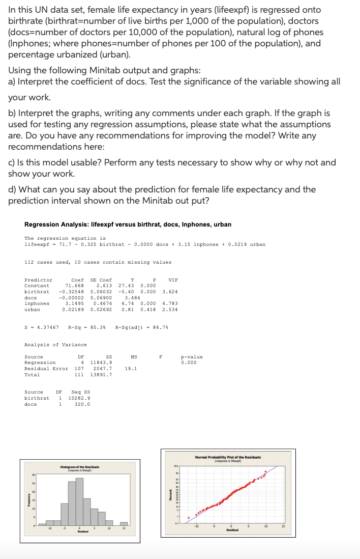
In this UN data set, female life expectancy in years (lifeexpf) is regressed onto birthrate (birthrat=number of live births per 1,000 of the population), doctors (docs=number of doctors per 10,000 of the population), natural log of phones (Inphones; where phones=number of phones per 100 of the population), and percentage urbanized (urban). Using the following Minitab output and graphs: a) Interpret the coefficient of docs. Test the significance of the variable showing all your work. b) Interpret the graphs, writing any comments under each graph. If the graph is used for testing any regression assumptions, please state what the assumptions are. Do you have any recommendations for improving the model? Write any recommendations here: c) Is this model usable? Perform any tests necessary to show why or why not and show your work. d) What can you say about the prediction for female life expectancy and the prediction interval shown on the Minitab out put? Regression Analysis: lifeexpf versus birthrat, docs, Inphones, urban The regression equation is lifeexpf - 71.7 - 0.325 birthrat - 0.0000 does + 3.15 Inphones + 0.0219 urban 112 cases used, 10 cases contain missing values Predictor Coef SE Coef P VIF Constant 71.668 2.613 27.43 0.000 birthrat -0.32548 0.06032 -5.40 0.000 3.624 docs -0.00002 0.06900 3.484 6.74 0.000 Inphones 3.1495 0.4674 4.783 urban 0.02189 0.02692 0.81 0.418 2.534 s - 4.37467 R-Sq - 85.3% R-Sq(adj) - 84.74 Analysis of Variance p-value 0.000 Source DE ss MS Regression Residual Error 107 Total 4 11843.9 2047.7 19.1 111 13891.7 Source DF Seg ss 1 10282.9 birthrat docs 1 320.0 Normal Probabity Plotof the Residals Hgramhe Residls
In this UN data set, female life expectancy in years (lifeexpf) is regressed onto birthrate (birthrat=number of live births per 1,000 of the population), doctors (docs=number of doctors per 10,000 of the population), natural log of phones (Inphones; where phones=number of phones per 100 of the population), and percentage urbanized (urban). Using the following Minitab output and graphs: a) Interpret the coefficient of docs. Test the significance of the variable showing all your work. b) Interpret the graphs, writing any comments under each graph. If the graph is used for testing any regression assumptions, please state what the assumptions are. Do you have any recommendations for improving the model? Write any recommendations here: c) Is this model usable? Perform any tests necessary to show why or why not and show your work. d) What can you say about the prediction for female life expectancy and the prediction interval shown on the Minitab out put? Regression Analysis: lifeexpf versus birthrat, docs, Inphones, urban The regression equation is lifeexpf - 71.7 - 0.325 birthrat - 0.0000 does + 3.15 Inphones + 0.0219 urban 112 cases used, 10 cases contain missing values Predictor Coef SE Coef P VIF Constant 71.668 2.613 27.43 0.000 birthrat -0.32548 0.06032 -5.40 0.000 3.624 docs -0.00002 0.06900 3.484 6.74 0.000 Inphones 3.1495 0.4674 4.783 urban 0.02189 0.02692 0.81 0.418 2.534 s - 4.37467 R-Sq - 85.3% R-Sq(adj) - 84.74 Analysis of Variance p-value 0.000 Source DE ss MS Regression Residual Error 107 Total 4 11843.9 2047.7 19.1 111 13891.7 Source DF Seg ss 1 10282.9 birthrat docs 1 320.0 Normal Probabity Plotof the Residals Hgramhe Residls

Chapter6: Exponential And Logarithmic Functions
Section6.8: Fitting Exponential Models To Data
Problem 3TI: Table 6 shows the population, in thousands, of harbor seals in the Wadden Sea over the years 1997 to...

Related questions
Question
Transcribed Image Text:In this UN data set, female life expectancy in years (lifeexpf) is regressed onto
birthrate (birthrat=number of live births per 1,000 of the population), doctors
(docs=number of doctors per 10,000 of the population), natural log of phones
(Inphones; where phones=number of phones per 100 of the population), and
percentage urbanized (urban).
Using the following Minitab output and graphs:
a) Interpret the coefficient of docs. Test the significance of the variable showing all
your work.
b) Interpret the graphs, writing any comments under each graph. If the graph is
used for testing any regression assumptions, please state what the assumptions
are. Do you have any recommendations for improving the model? Write any
recommendations here:
c) Is this model usable? Perform any tests necessary to show why or why not and
show your work.
d) What can you say about the prediction for female life expectancy and the
prediction interval shown on the Minitab out put?
Regression Analysis: lifeexpf versus birthrat, docs, Inphones, urban
The regression equation is
lifeexpf - 71.7 - 0.325 birthrat - 0.0000 docs + 3.15 Inphones + 0.0219 urban
112 cases used, 10 cases contain missing values
SE Coef
2.613
Predictor
Coef
T
P
VIF
Constant
71.668
27.43 0.00o
birthrat
-0.32548
0.06032
-5.40 0.000
3.624
0.06900
0.4674
docs
-0.00002
3.1495
3.484
Inphones
urban
6.74
0.000 4.783
0.02189
0.02692
0.81
0.418 2.534
s - 4.37467
R-Sq - 85.3%
R-Sq (adj) - 84.7%
Analysis of Variance
p-value
0.000
Source
DF
s
MS
Regression
4 11843.9
2047.7
13891.7
Residual Error
107
19.1
Total
111
Seq ss
10282.9
Source
DF
birthrat
1
docs
1
320.0
Normel Probability Plot of the Residuals
(resporse isee)
Histogramof tthe Residuals
mpore ee
10
15
Residual
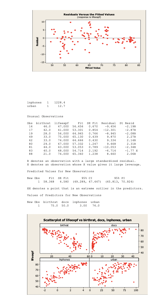
Transcribed Image Text:Residuals Versus the Fitted Values
(response is lifeexp)
10-
5-
-5-
10-
-15-
50
55
60
65
75
80
70
Fitted Value
85
Inphones
urban
1
1228.4
1
12.7
Unusual Observations
Obs
birthrat
46.0
lifeexpf
47.000
41.000
56.000
75.000
Fit
SE Fit
Residual
-9.456
St Resid
-2.19R
14
56.456
0.670
-12.301
-8.945
9.870
17
42.0
53.301
0.854
-2.87R
-2.08R
2.27R
19
28.0
64.945
65.130
0.766
49
33.0
0.439
2.14R
2.31R
-2.34R
62
33.0
74.000
64.666
0.430
9.334
80
29.0
67.000
57.332
1.247
9.668
81
44.0
43.000 53.053
0.789
-10.053
-6.714
8.660
83
40.0
48.000
54.714
2.192
-1.77 X
88
21.0
74.000
65.340
1.238
2.06R
R denotes an observation with a large standardized residual.
x denotes an observation whose X value gives it large leverage.
Predicted Values for New Observations
New Obs
Fit SE Fit
95% CI
95% PI
1
58.368
4.580
(49.289, 67.447)
(45.813, 70.924)
Xx denotes a point that is an extreme outlier in the predictors.
Values of Predictors for New Observations
New Obs
birthrat
docs
75.0 50.0
Inphones
3.00
urban
1
76.0
Scatterplot of lifeexpf vs birthrat, docs, Inphones, urban
birthrat
docs
•
80
70
-60
50
40
20
60 0
10
20
30
40
Inphones
40
urban
80
70
60-
50
40
2
25
50
75
100
Expert Solution
This question has been solved!
Explore an expertly crafted, step-by-step solution for a thorough understanding of key concepts.

This is a popular solution!

Trending now
This is a popular solution!

Step by step
Solved in 4 steps

Recommended textbooks for you

Algebra & Trigonometry with Analytic Geometry
Algebra
ISBN:
9781133382119
Author:
Swokowski
Publisher:
Cengage

Elementary Linear Algebra (MindTap Course List)
Algebra
ISBN:
9781305658004
Author:
Ron Larson
Publisher:
Cengage Learning
Algebra & Trigonometry with Analytic Geometry
Algebra
ISBN:
9781133382119
Author:
Swokowski
Publisher:
Cengage
Elementary Linear Algebra (MindTap Course List)
Algebra
ISBN:
9781305658004
Author:
Ron Larson
Publisher:
Cengage Learning