The following table lists a portion of Major League Baseball’s (MLB’s) leading pitchers, each pitcher’s salary (In $ millions), and earned run average (ERA) for 2008. Salary ERA J. Santana 10.0 2.49 C. Lee 4.0 2.30 ⋮ ⋮ ⋮ C. Hamels 0.5 2.75


All but A-2 please
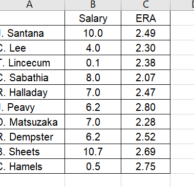
The following table lists a portion of Major League Baseball’s (MLB’s) leading pitchers, each pitcher’s salary (In $ millions), and earned run average (ERA) for 2008.
| Salary | ERA | |||||
| J. Santana | 10.0 | 2.49 | ||||
| C. Lee | 4.0 | 2.30 | ||||
| ⋮ | ⋮ | ⋮ | ||||
| C. Hamels | 0.5 | 2.75 | ||||
Click here for the Excel Data File
a-1. Estimate the model: Salary = β0 + β1ERA + ε. (Negative values should be indicated by a minus sign. Enter your answers, in millions, rounded to 2 decimal places.)
Salaryˆ=Salary^= + ERA
a-2. Interpret the coefficient of ERA.
multiple choice
-
A one-unit increase in ERA, predicted salary decreases by $0.99 million. Correct
-
A one-unit increase in ERA, predicted salary increases by $0.99 million.
-
A one-unit increase in ERA, predicted salary decreases by $7.43 million.
-
A one-unit increase in ERA, predicted salary increases by $7.43 million.
b. Use the estimated model to predict salary for each player, given his ERA. For example, use the sample regression equation to predict the salary for J. Santana with ERA = 2.49. (Round coefficient estimates to at least 4 decimal places and final answers, in millions, to 2 decimal places.)
c. Derive the corresponding residuals. (Negative values should be indicated by a minus sign. Round coefficient estimates to at least 4 decimal places and final answers, in millions, to 2 decimal places.)


Trending now
This is a popular solution!

Step by step
Solved in 2 steps with 2 images


