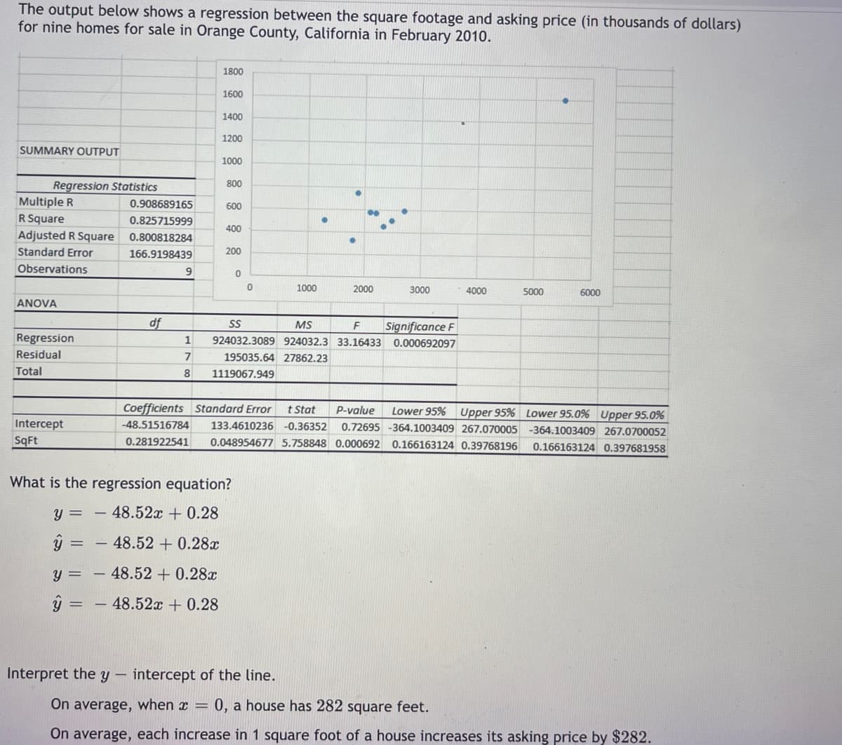
The output below shows a regression between the square footage and asking price (in thousands of dollars) for nine homes for sale in Orange County, California in February 2010. 1800 1600 1400 1200 SUMMARY OUTPUT 1000 800 Regression Statistics Multiple R 0.908689165 600 R Square 0.825715999 400 Adjusted R Square 0.800818284 Standard Error 166.9198439 200 Observations 9 1000 2000 3000 4000 5000 6000 ANOVA df SS Significance F 924032.3089 924032.3 33.16433 0.000692097 MS F Regression Residual 195035.64 27862.23 Total 8 1119067.949 Coefficients Standard Error t Stat P-value Lower 95% Upper 95% Lower 95.0% Upper 95.0% Intercept -48.51516784 133.4610236 -0.36352 0.72695 -364.1003409 267.070005 -364.1003409 267.0700052 Sqft 0.281922541 0.048954677 5.758848 0.000692 0.166163124 0.39768196 0.166163124 0.397681958 What is the regression equation? y = 48.52x + 0.28 48.52 + 0.28x y = – 48.52 + 0.28x 48.52x +0.28 Interpret the y – intercept of the line. On average, when x = 0, a house has 282 square feet. On average, each increase in 1 square foot of a house increases its asking price by $282
The output below shows a regression between the square footage and asking price (in thousands of dollars) for nine homes for sale in Orange County, California in February 2010. 1800 1600 1400 1200 SUMMARY OUTPUT 1000 800 Regression Statistics Multiple R 0.908689165 600 R Square 0.825715999 400 Adjusted R Square 0.800818284 Standard Error 166.9198439 200 Observations 9 1000 2000 3000 4000 5000 6000 ANOVA df SS Significance F 924032.3089 924032.3 33.16433 0.000692097 MS F Regression Residual 195035.64 27862.23 Total 8 1119067.949 Coefficients Standard Error t Stat P-value Lower 95% Upper 95% Lower 95.0% Upper 95.0% Intercept -48.51516784 133.4610236 -0.36352 0.72695 -364.1003409 267.070005 -364.1003409 267.0700052 Sqft 0.281922541 0.048954677 5.758848 0.000692 0.166163124 0.39768196 0.166163124 0.397681958 What is the regression equation? y = 48.52x + 0.28 48.52 + 0.28x y = – 48.52 + 0.28x 48.52x +0.28 Interpret the y – intercept of the line. On average, when x = 0, a house has 282 square feet. On average, each increase in 1 square foot of a house increases its asking price by $282

Glencoe Algebra 1, Student Edition, 9780079039897, 0079039898, 2018
18th Edition
ISBN:9780079039897
Author:Carter
Publisher:Carter
Chapter4: Equations Of Linear Functions
Section4.5: Correlation And Causation
Problem 2CYU

Related questions
Question
Transcribed Image Text:The output below shows a regression between the square footage and asking price (in thousands of dollars)
for nine homes for sale in Orange County, California in February 2010.
1800
1600
1400
1200
SUMMARY OUTPUT
1000
Regression Statistics
800
Multiple R
0.908689165
600
R Square
0.825715999
400
Adjusted R Square
0.800818284
Standard Error
166.9198439
200
Observations
1000
2000
3000
4000
5000
6000
ANOVA
df
Significance F
924032.3089 924032.3 33.16433 0.000692097
MS
Regression
1
Residual
7
195035.64 27862.23
Total
8
1119067.949
Coefficients Standard Error
t Stat
P-value
Lower 95% Upper 95% Lower 95.0% Upper 95.0%
Intercept
-48.51516784
133.4610236 -0.36352
0.72695 -364.1003409 267.070005 -364.1003409 267.0700052
Sqft
0.281922541
0.048954677 5.758848 0.000692 0.166163124 0.39768196
0.166163124 0.397681958
What is the regression equation?
y =
48.52x + 0.28
- 48.52 + 0.28x
y =
48.52 + 0.28x
48.52x +0.28
Interpret the y –
intercept of the line.
On average, when x =
0, a house has 282 square feet.
On average, each increase in 1 square foot of a house increases its asking price by $282.
Transcribed Image Text:On
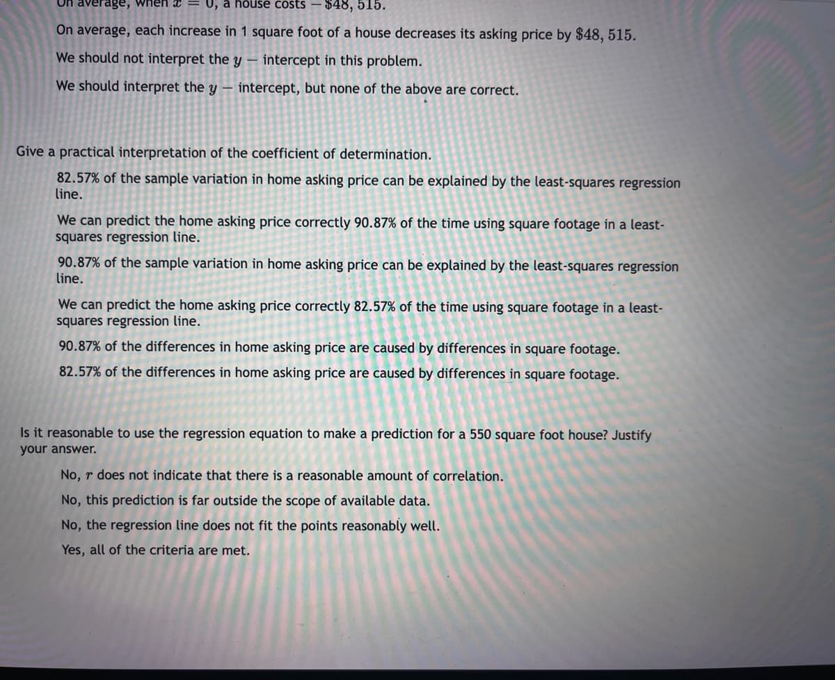
rage, when x = U, a house costs –$48, 515.
On average, each increase in 1 square foot of a house decreases its asking price by $48, 515.
We should not interpret the y –
intercept in this problem.
We should interpret the y – intercept, but none of the above are correct.
Give a practical interpretation of the coefficient of determination.
82.57% of the sample variation in home asking price can be explained by the least-squares regression
line.
We can predict the home asking price correctly 90.87% of the time using square footage in a least-
squares regression line.
90.87% of the sample variation in home asking price can be explained by the least-squares regression
line.
We can predict the home asking price correctly 82.57% of the time using square footage in a least-
squares regression line.
90.87% of the differences in home asking price are caused by differences in square footage.
82.57% of the differences in home asking price are caused by differences in square footage.
Is it reasonable to use the regression equation to make a prediction for a 550 square foot house? Justify
your answer.
No, r does not indicate that there is a reasonable amount of correlation.
No, this prediction is far outside the scope of available data.
No, the regression line does not fit the points reasonably well.
Yes, all of the criteria are met.
Expert Solution
This question has been solved!
Explore an expertly crafted, step-by-step solution for a thorough understanding of key concepts.

This is a popular solution!

Trending now
This is a popular solution!

Step by step
Solved in 2 steps

Recommended textbooks for you
Glencoe Algebra 1, Student Edition, 9780079039897…
Algebra
ISBN:
9780079039897
Author:
Carter
Publisher:
McGraw Hill

Linear Algebra: A Modern Introduction
Algebra
ISBN:
9781285463247
Author:
David Poole
Publisher:
Cengage Learning

Functions and Change: A Modeling Approach to Coll…
Algebra
ISBN:
9781337111348
Author:
Bruce Crauder, Benny Evans, Alan Noell
Publisher:
Cengage Learning
Glencoe Algebra 1, Student Edition, 9780079039897…
Algebra
ISBN:
9780079039897
Author:
Carter
Publisher:
McGraw Hill
Linear Algebra: A Modern Introduction
Algebra
ISBN:
9781285463247
Author:
David Poole
Publisher:
Cengage Learning
Functions and Change: A Modeling Approach to Coll…
Algebra
ISBN:
9781337111348
Author:
Bruce Crauder, Benny Evans, Alan Noell
Publisher:
Cengage Learning