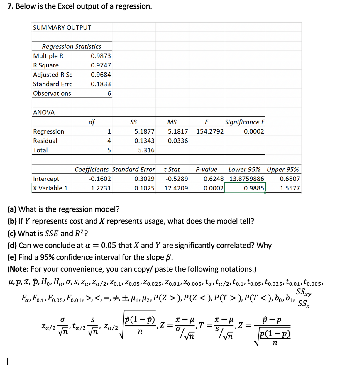
7. Below is the Excel output of a regression. SUMMARY OUTPUT Regression Statistics Multiple R 0.9873 R Square 0.9747 Adjusted R Sc 0.9684 Standard Errc 0.1833 Observations 6 ANOVA df SS MS Significance F Regression 5.1877 5.1817 154.2792 0.0002 Residual 4 0.1343 0.0336 Total 5 5.316 Coefficients Standard Error t Stat P-value Lower 95% Upper 95% Intercept -0.1602 0.3029 -0.5289 0.6248 13.8759886 0.6807 X Variable 1 1.2731 0.1025 12.4209 0.0002 0.9885 1.5577 (a) What is the regression model? (b) If Y represents cost and X represents usage, what does the model tell? (c) What is SSE and R2? (d) Can we conclude at a = 0.05 that X and Y are significantly correlated? Why (e) Find a 95% confidence interval for the slope ß.

Which of the following situations could produce data sets or plots that could have a regression line with a negative y-intercept? Select all that apply.   Select all that apply: The net profit of a company as a function of the number of months since it was founded, where net income is gross income minus expenses. The number of employees of a company as a function of the number of months since it was founded. The cost of a company's flagship product as a function of the number of months since it was founded. The number of franchises of a company as a function of the number of months since it was founded.

It is a 2 part question. How can we find normality?

Consider a regression model. The coefficient of determination (R2) gives the proportion of the variability in the dependent variable that is explained by the regression equation.   True False

On the first day of class, an economics professor administers a test to gauge the math preparedness of her students. She believes that the performance on this math test and the number of hours studied per week on the course are the primary factors that predict a student's score on the final exam. Using data from her class of 60 students, she estimates   A portion of the regression results is shown in the following table. a. What is the slope coefficient of Hours? b. What is the sample regression equation? c. What is the predicted final exam score for a student who has a math score of 70 and studies 4 hours per week?

c. What are the 2 main pieces of information you get from the linear regression model? Should I go back to the data set and recalculate slope and y intercept if I already have determined the equation of the trend line?

Hello, the attached picture is the background information for the posted question. Thank you! 2e. Calculate the Rsq of the regression and interpret the Rsq.

The accompanying data are the number of wins and the earned run averages (mean number of earned runs allowed per nine innings pitched) for eight baseball pitchers in a recent season. Find the equation of the regression line. Then construct a scatter plot of the data and draw the regression line. Then use the regression equation to predict the value of y for each of the given x-values, if meaningful. If the x-value is not meaningful to predict the value of y, explain why not. (a) x= 5 wins E Click the icon to view the table of numbers of wins and earned run average. (b) x = 10 wins (c) x = 19 wins (d) x= 15 wins ..... The equation of the regression line is y = x+O (Round to two decimal places as needed.) Wins and ERA Earned run Wins, x average, y 20 2.71 18 3.19 17 2.69 16 3.68 14 3.94 12 4.25 11 3.86 9 5.18 Print Done

We wants to assess the relationship between overall GPA (4.0 scale) and amount of time spent weekly on school work of 50 college students. Simple linear regression model is used and some results for the model is given: a) Is it plausible that the true intercept for the model is 2.0? Why or why not? (hint: using interval for intercept) b) If 2.0 is the real intercept for the model, does it make contextual sense? Explain why it is or why it is not. c) Using the model, calculate the number of hours needed to achieve a GPA of 4.0. Then explain why this estimate number of hours is biased. (hint: think about Y).

A graphing calculator is recommended. When laboratory rats are exposed to asbestos fibers, some of them develop lung tumors. The table lists the results of several experiments by different scientists. Asbestos exposure (fibers/mL) y = 50 Mice with Tumors (%) 400 O 500 900 1,100 1,600 1,800 2,000 3,000 3000 2500 2000 1500 (a) Find the regression line for the data. (Use x for asbestos exposure in fibers/mL and y for percent of mice with tumors. Round your values to four decimal places.) 1000 500 Percent of mice that develop lung tumors (b) Construct a scatter plot and graph the regression line. o 0 7 6 11 10 27 41 38 37 49 20 30 40 50 Asbestos Exposure (Fibers/mL.) 60 Mice with Tumors (%) 3000 ● 2500 2000 1500 1000 500 60 0 0 10 20 30 40 50 60 Asbestos Exposure (Fibers/mL) Ⓡ 4