In this tutorial you are tasked with using this Monte Carlo integration method to estimate the values of the following integrals: 11 =Lxdx =0 12 = = S² 2 πT e² + 13 = L cos(x) e² dx = 1+2 You may not make use of any integration methods from other packages. For the integration method you are only allowed to make use of NumPy. This tutorial contains many questions. These are largely rhetorical, so you do not need to write answers to them. Please ensure that you follow all the instructions to produce the desired plots (one per part). Ask the lecturer or tutors if you are unsure of what is expected of you in any part. For this tutorial, you may find it useful to read the section on NumPy Conditional Statements and np. where from the NumPy chapter of the notes. Part 1 Before you start integrating, illustrate the first few steps of the process by generating a set of random points in the appropriate boundaries for each integral (consider what these boundaries should be), and plotting these points along with the curve for each integrand function, and a line for the x-axis. In this plot use different styles for points inside the area of integration, and those outside this area. Make sure to label these points appropriately. Do not use so many points that you can no longer distinguish individual ones. You may use a single plot with subplots, or a plot for each integral. For the name(s) of your plots use: tut4_p1_lx_student_number.png, where x is the number assigned to the integral (if you have multiple integrands in one plot, use each number in sequence, e.g. "tut4_p1_1123_student_number.png" for all 3 in one plot). Tutorial 4 - Monte Carlo Integration Note, although this tutorial is presented in many parts, you may use a single script or notebook for your solutions. In this tutorial you will explore a Monte Carlo integration method. Monte Carlo methods are a class of numerical methods that make use of random sampling, named after the famous casino / city. In this method the integral of a one-dimensional, one-to-one function f(x) is estimated by: Generating M uniformly sampled random points in a rectangular region containing the integration limits and the limits of the function. Counting the number of points between the function and the x-axis, above the x-axis ( M+) and below the x-axis (M) separately. Estimating the area between the x-axis and the function (the value of the integral) using the ratio (MM)/M and equating it to the ratio of the ear of integration (I) and the total area of the regionA: I/A. This provides the formula: (Mo - Mo) I= A- M This is illustrated in the figure below, where the area that is highlighted is the result from integration, the interval of the integral (and the a boundaries of the random points) are (a, b) and the bounds chosen for the y-axis to ensure that the function is contained in the integration interval interval is (a,b). The randomly generated points are represented by X for points outside the area of integration, and by for those inside the area of integration; note that these points are all generated from the same set of random values. Ул Ур Area of integral × Points outside O Points inside Ya Xale e × × Θ f(x)
In this tutorial you are tasked with using this Monte Carlo integration method to estimate the values of the following integrals: 11 =Lxdx =0 12 = = S² 2 πT e² + 13 = L cos(x) e² dx = 1+2 You may not make use of any integration methods from other packages. For the integration method you are only allowed to make use of NumPy. This tutorial contains many questions. These are largely rhetorical, so you do not need to write answers to them. Please ensure that you follow all the instructions to produce the desired plots (one per part). Ask the lecturer or tutors if you are unsure of what is expected of you in any part. For this tutorial, you may find it useful to read the section on NumPy Conditional Statements and np. where from the NumPy chapter of the notes. Part 1 Before you start integrating, illustrate the first few steps of the process by generating a set of random points in the appropriate boundaries for each integral (consider what these boundaries should be), and plotting these points along with the curve for each integrand function, and a line for the x-axis. In this plot use different styles for points inside the area of integration, and those outside this area. Make sure to label these points appropriately. Do not use so many points that you can no longer distinguish individual ones. You may use a single plot with subplots, or a plot for each integral. For the name(s) of your plots use: tut4_p1_lx_student_number.png, where x is the number assigned to the integral (if you have multiple integrands in one plot, use each number in sequence, e.g. "tut4_p1_1123_student_number.png" for all 3 in one plot). Tutorial 4 - Monte Carlo Integration Note, although this tutorial is presented in many parts, you may use a single script or notebook for your solutions. In this tutorial you will explore a Monte Carlo integration method. Monte Carlo methods are a class of numerical methods that make use of random sampling, named after the famous casino / city. In this method the integral of a one-dimensional, one-to-one function f(x) is estimated by: Generating M uniformly sampled random points in a rectangular region containing the integration limits and the limits of the function. Counting the number of points between the function and the x-axis, above the x-axis ( M+) and below the x-axis (M) separately. Estimating the area between the x-axis and the function (the value of the integral) using the ratio (MM)/M and equating it to the ratio of the ear of integration (I) and the total area of the regionA: I/A. This provides the formula: (Mo - Mo) I= A- M This is illustrated in the figure below, where the area that is highlighted is the result from integration, the interval of the integral (and the a boundaries of the random points) are (a, b) and the bounds chosen for the y-axis to ensure that the function is contained in the integration interval interval is (a,b). The randomly generated points are represented by X for points outside the area of integration, and by for those inside the area of integration; note that these points are all generated from the same set of random values. Ул Ур Area of integral × Points outside O Points inside Ya Xale e × × Θ f(x)

Database System Concepts
7th Edition
ISBN:9780078022159
Author:Abraham Silberschatz Professor, Henry F. Korth, S. Sudarshan
Publisher:Abraham Silberschatz Professor, Henry F. Korth, S. Sudarshan
Chapter1: Introduction
Section: Chapter Questions
Problem 1PE

Related questions
Question
Solve these questions
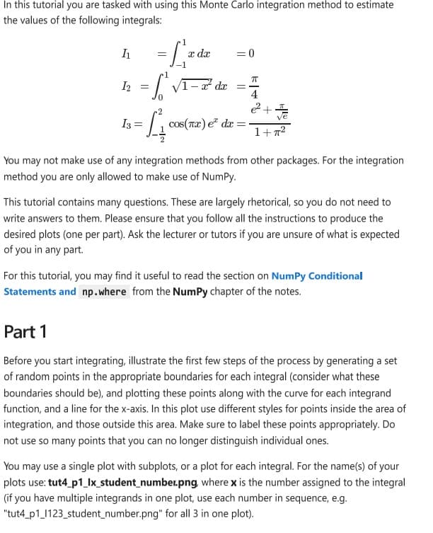
Transcribed Image Text:In this tutorial you are tasked with using this Monte Carlo integration method to estimate
the values of the following integrals:
11
=Lxdx
=0
12 =
= S²
2
πT
e² +
13 =
L
cos(x) e² dx =
1+2
You may not make use of any integration methods from other packages. For the integration
method you are only allowed to make use of NumPy.
This tutorial contains many questions. These are largely rhetorical, so you do not need to
write answers to them. Please ensure that you follow all the instructions to produce the
desired plots (one per part). Ask the lecturer or tutors if you are unsure of what is expected
of you in any part.
For this tutorial, you may find it useful to read the section on NumPy Conditional
Statements and np. where from the NumPy chapter of the notes.
Part 1
Before you start integrating, illustrate the first few steps of the process by generating a set
of random points in the appropriate boundaries for each integral (consider what these
boundaries should be), and plotting these points along with the curve for each integrand
function, and a line for the x-axis. In this plot use different styles for points inside the area of
integration, and those outside this area. Make sure to label these points appropriately. Do
not use so many points that you can no longer distinguish individual ones.
You may use a single plot with subplots, or a plot for each integral. For the name(s) of your
plots use: tut4_p1_lx_student_number.png, where x is the number assigned to the integral
(if you have multiple integrands in one plot, use each number in sequence, e.g.
"tut4_p1_1123_student_number.png" for all 3 in one plot).
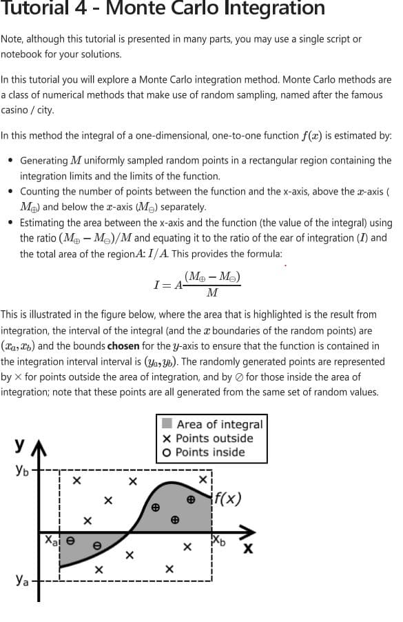
Transcribed Image Text:Tutorial 4 - Monte Carlo Integration
Note, although this tutorial is presented in many parts, you may use a single script or
notebook for your solutions.
In this tutorial you will explore a Monte Carlo integration method. Monte Carlo methods are
a class of numerical methods that make use of random sampling, named after the famous
casino / city.
In this method the integral of a one-dimensional, one-to-one function f(x) is estimated by:
Generating M uniformly sampled random points in a rectangular region containing the
integration limits and the limits of the function.
Counting the number of points between the function and the x-axis, above the x-axis (
M+) and below the x-axis (M) separately.
Estimating the area between the x-axis and the function (the value of the integral) using
the ratio (MM)/M and equating it to the ratio of the ear of integration (I) and
the total area of the regionA: I/A. This provides the formula:
(Mo - Mo)
I= A-
M
This is illustrated in the figure below, where the area that is highlighted is the result from
integration, the interval of the integral (and the a boundaries of the random points) are
(a, b) and the bounds chosen for the y-axis to ensure that the function is contained in
the integration interval interval is (a,b). The randomly generated points are represented
by X for points outside the area of integration, and by for those inside the area of
integration; note that these points are all generated from the same set of random values.
Ул
Ур
Area of integral
× Points outside
O Points inside
Ya
Xale
e
×
×
Θ
f(x)
AI-Generated Solution

Unlock instant AI solutions
Tap the button
to generate a solution
Recommended textbooks for you
Database System Concepts
Computer Science
ISBN:
9780078022159
Author:
Abraham Silberschatz Professor, Henry F. Korth, S. Sudarshan
Publisher:
McGraw-Hill Education

Starting Out with Python (4th Edition)
Computer Science
ISBN:
9780134444321
Author:
Tony Gaddis
Publisher:
PEARSON

Digital Fundamentals (11th Edition)
Computer Science
ISBN:
9780132737968
Author:
Thomas L. Floyd
Publisher:
PEARSON
Database System Concepts
Computer Science
ISBN:
9780078022159
Author:
Abraham Silberschatz Professor, Henry F. Korth, S. Sudarshan
Publisher:
McGraw-Hill Education
Starting Out with Python (4th Edition)
Computer Science
ISBN:
9780134444321
Author:
Tony Gaddis
Publisher:
PEARSON
Digital Fundamentals (11th Edition)
Computer Science
ISBN:
9780132737968
Author:
Thomas L. Floyd
Publisher:
PEARSON

C How to Program (8th Edition)
Computer Science
ISBN:
9780133976892
Author:
Paul J. Deitel, Harvey Deitel
Publisher:
PEARSON

Database Systems: Design, Implementation, & Manag…
Computer Science
ISBN:
9781337627900
Author:
Carlos Coronel, Steven Morris
Publisher:
Cengage Learning

Programmable Logic Controllers
Computer Science
ISBN:
9780073373843
Author:
Frank D. Petruzella
Publisher:
McGraw-Hill Education