Unstandardized Coefficients B t Std. Error 1 (Constant) Sig. .000 12.423 .164 75.752 Mothers highest degree 1.117 .101 .416 .000 11.024 a. Respondents sex = FEMALE b. Dependent Variable: Highest year of school completed C10. In Exercise 6, we examined the relationship between years of education and hours of television watched per day. We saw that as education increases, hours of television viewing decreases. The number of children a family has could also affect how much television is viewed per day. Having children may lead to more shared and supervised viewing and thus increases the number of viewing hours. The following SPSS output displays the relationship between television viewing (measured in hours per day) and both education (measured in years) and number of children. We hypothesize that whereas more education may lead to less viewing, the number of children has the opposite effect: Having more children will result in more hours of viewing per day. a. What is the b coefficient for education? For number of children? Interpret each coefficient. Is the relationship between each independent variable and hours of viewing as hypothesized? b. Using the multiple regression equation with both education and number of children as independent variables, calculate the number of hours of television viewing for Standardized Coefficients Beta
Unstandardized Coefficients B t Std. Error 1 (Constant) Sig. .000 12.423 .164 75.752 Mothers highest degree 1.117 .101 .416 .000 11.024 a. Respondents sex = FEMALE b. Dependent Variable: Highest year of school completed C10. In Exercise 6, we examined the relationship between years of education and hours of television watched per day. We saw that as education increases, hours of television viewing decreases. The number of children a family has could also affect how much television is viewed per day. Having children may lead to more shared and supervised viewing and thus increases the number of viewing hours. The following SPSS output displays the relationship between television viewing (measured in hours per day) and both education (measured in years) and number of children. We hypothesize that whereas more education may lead to less viewing, the number of children has the opposite effect: Having more children will result in more hours of viewing per day. a. What is the b coefficient for education? For number of children? Interpret each coefficient. Is the relationship between each independent variable and hours of viewing as hypothesized? b. Using the multiple regression equation with both education and number of children as independent variables, calculate the number of hours of television viewing for Standardized Coefficients Beta

Algebra & Trigonometry with Analytic Geometry
13th Edition
ISBN:9781133382119
Author:Swokowski
Publisher:Swokowski
Chapter3: Functions And Graphs
Section3.3: Lines
Problem 76E

Related questions
Question
Question 10
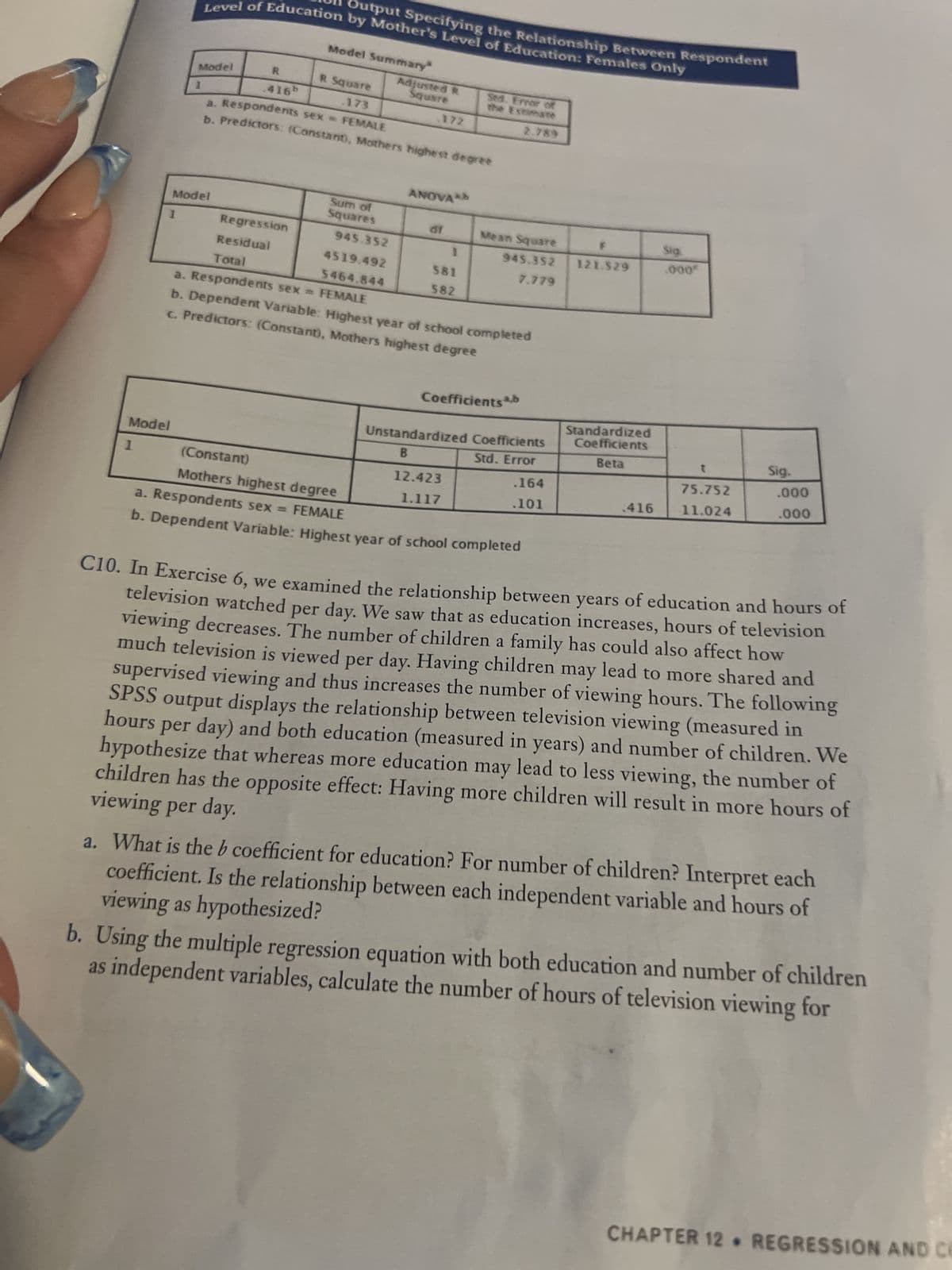
Transcribed Image Text:Level of Education by Mother's Level of Education: Females Only
Output Specifying the Relationship Between Respondent
Model Summary
Model
R
R Square
Adjusted R
Square
.416b
.173
Sed. Error of
the Estimate
2.789
172
a. Respondents sex = FEMALE
b. Predictors: (Constant), Mothers highest degree
ANOVA
Model
df
1
Regression
Residual
Sum of
Squares
945.352
4519.492
5464.844
Sig.
.000*
1
Total
581
582
a. Respondents sex = FEMALE
b. Dependent Variable: Highest year of school completed
c. Predictors: (Constant), Mothers highest degree
Coefficients ab
Unstandardized Coefficients
B
t
Model
Std. Error
Sig.
.000
.000
75.752
1
(Constant)
12.423
.164
11.024
.416
Mothers highest degree
1.117
.101
a. Respondents sex = FEMALE
b. Dependent Variable: Highest year of school completed
C10. In Exercise 6, we examined the relationship between years of education and hours of
television watched per day. We saw that as education increases, hours of television
viewing decreases. The number of children a family has could also affect how
much television is viewed per day. Having children may lead to more shared and
supervised viewing and thus increases the number of viewing hours. The following
SPSS output displays the relationship between television viewing (measured in
hours per day) and both education (measured in years) and number of children. We
hypothesize that whereas more education may lead to less viewing, the number of
viewing per day.
children has the opposite effect: Having more children will result in more hours of
a. What is the b coefficient for education? For number of children? Interpret each
viewing as hypothesized?
coefficient. Is the relationship between each independent variable and hours of
b. Using the multiple regression equation with both education and number of children
as independent variables, calculate the number of hours of television viewing for
Mean Square
945.352 121.529
7.779
Standardized
Coefficients
Beta
CHAPTER 12. REGRESSION AND CE
Transcribed Image Text:BE
VALU
WINNER
e
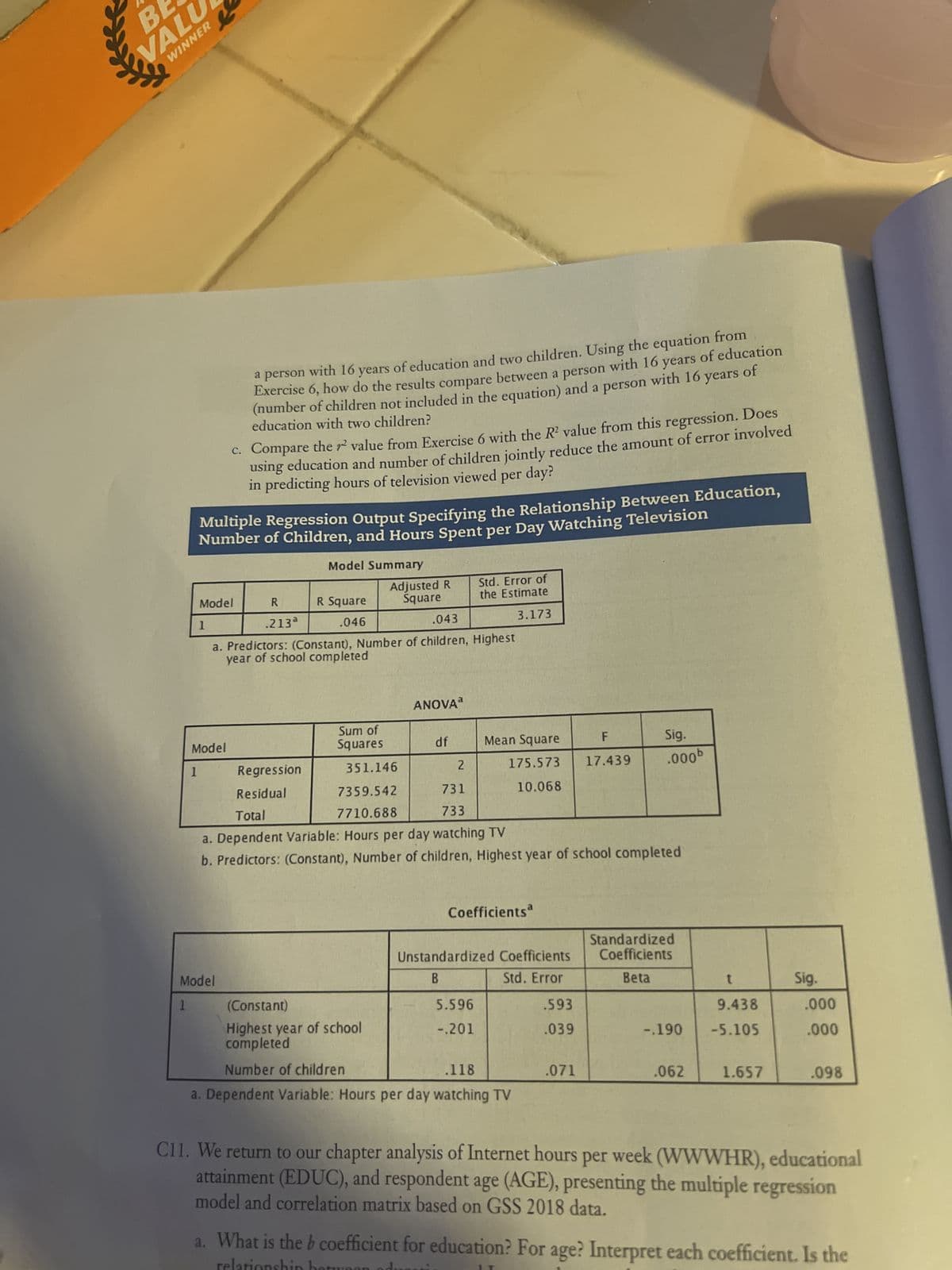
a person with 16 years of education and two children. Using the equation from
Exercise 6, how do the results compare between a person with 16 years of education
(number of children not included in the equation) and a person with 16 years of
education with two children?
c. Compare the value from Exercise 6 with the R² value from this regression. Does
using education and number of children jointly reduce the amount of error involved
in predicting hours of television viewed per day?
Multiple Regression Output Specifying the Relationship Between Education,
Number of Children, and Hours Spent per Day Watching Television
Model Summary
Adjusted R
Square
Std. Error of
the Estimate
Model
R
.213ª
R Square
.046
3.173
1
.043
a. Predictors: (Constant), Number of children, Highest
year of school completed
ANOVA
F
Mean Square
Model
Sig.
.000b
17.439
Regression
1
Sum of
Squares
df
351.146
7359.542
7710.688
175.573
10.068
2
731
733
Residual
Total
a. Dependent Variable: Hours per day watching TV
b. Predictors: (Constant), Number of children, Highest year of school completed
Coefficients
Standardized
Coefficients
Unstandardized Coefficients
B
Model
Std. Error
Beta
t
1
(Constant)
5.596
.593
9.438
Highest year of school
completed
-.201
.039
-.190 -5.105
Number of children
.118
.071
.062
1.657
.098
a. Dependent Variable: Hours per day watching TV
C11. We return to our chapter analysis of Internet hours per week (WWWHR), educational
attainment (EDUC), and respondent age (AGE), presenting the multiple regression
model and correlation matrix based on GSS 2018 data.
relatio
a. What is the b coefficient for education? For age? Interpret each coefficient. Is the
Sig.
.000
.000
Expert Solution
This question has been solved!
Explore an expertly crafted, step-by-step solution for a thorough understanding of key concepts.

Step by step
Solved in 2 steps with 2 images

Recommended textbooks for you
Algebra & Trigonometry with Analytic Geometry
Algebra
ISBN:
9781133382119
Author:
Swokowski
Publisher:
Cengage

Glencoe Algebra 1, Student Edition, 9780079039897…
Algebra
ISBN:
9780079039897
Author:
Carter
Publisher:
McGraw Hill
Algebra & Trigonometry with Analytic Geometry
Algebra
ISBN:
9781133382119
Author:
Swokowski
Publisher:
Cengage
Glencoe Algebra 1, Student Edition, 9780079039897…
Algebra
ISBN:
9780079039897
Author:
Carter
Publisher:
McGraw Hill