One-way ANOVA Conditions Observations in each group is a random sample from a Normal population. • All populations have the same variance. Assumption considered reasonable if the largest sample SD is no larger than twice the smallest sample SD. • Samples are independent. • Normality assumption may be waived if each sample is greater than 20. Results are considered approximate question-Does it seem reasonable to make the assumptions needed to use the ANOVA procedure for these data? Justify your answer by referring to the above outputs. Produce the Density Trace and Normal Probability Plot of the Residuals.
One-way ANOVA Conditions Observations in each group is a random sample from a Normal population. • All populations have the same variance. Assumption considered reasonable if the largest sample SD is no larger than twice the smallest sample SD. • Samples are independent. • Normality assumption may be waived if each sample is greater than 20. Results are considered approximate question-Does it seem reasonable to make the assumptions needed to use the ANOVA procedure for these data? Justify your answer by referring to the above outputs. Produce the Density Trace and Normal Probability Plot of the Residuals.

MATLAB: An Introduction with Applications
6th Edition
ISBN:9781119256830
Author:Amos Gilat
Publisher:Amos Gilat
Chapter1: Starting With Matlab
Section: Chapter Questions
Problem 1P

Related questions
Topic Video
Question
One-way ANOVA
Conditions
Observations in each group is a random sample from a Normal population.
•
All populations have the same variance. Assumption considered reasonable if the largest sample SD is no larger than twice the smallest sample SD.
•
Samples are independent.
•
Normality assumption may be waived if each sample is greater than 20. Results are considered approximate
question-Does it seem reasonable to make the assumptions needed to use the ANOVA procedure for these data? Justify your answer by referring to the above outputs. Produce the Density Trace and Normal Probability Plot of the Residuals.
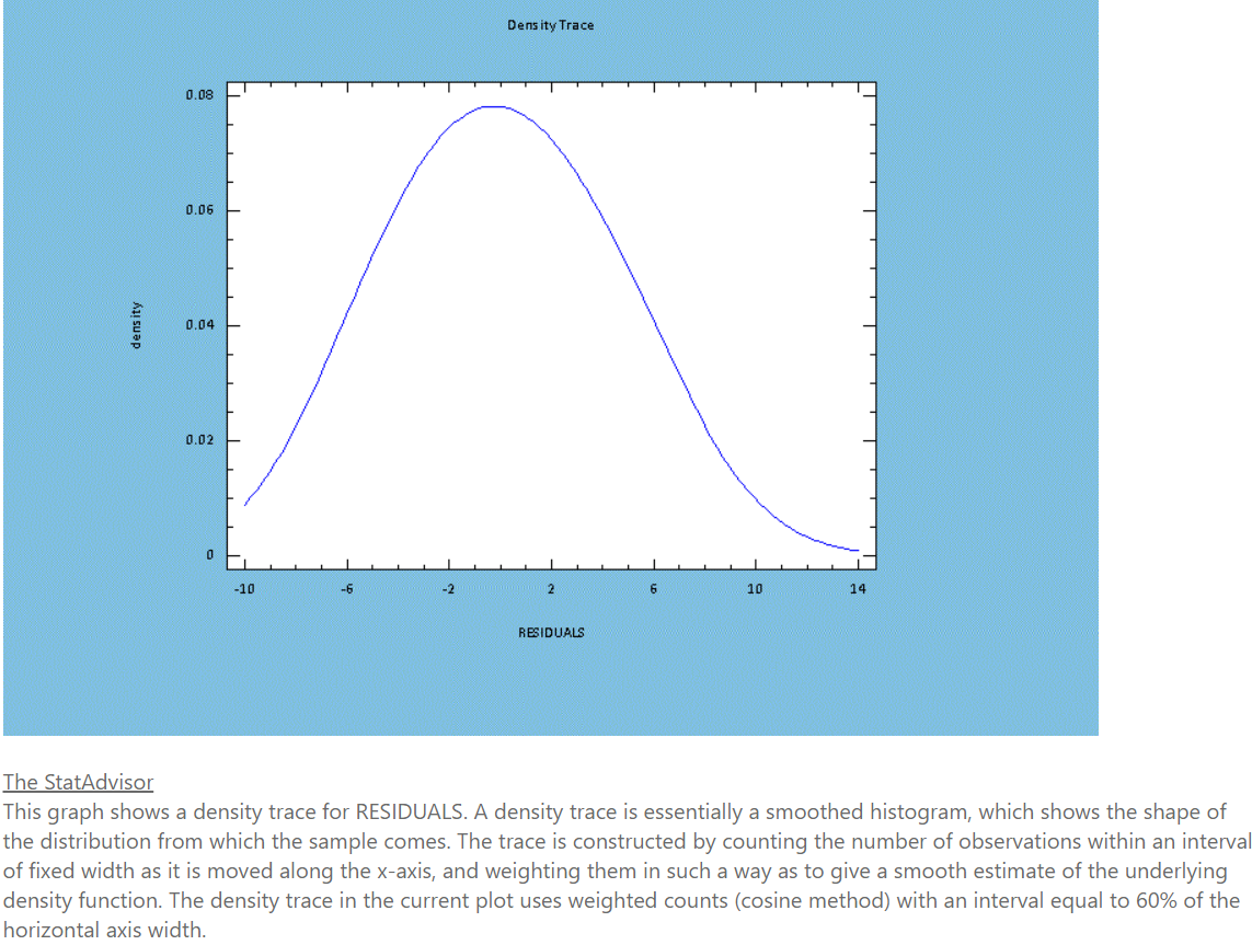
Transcribed Image Text:Dens ity Trace
0.08
0.06
0.04
0.02
-10
-6
-2
6
10
14
RESIDUALS
The StatAdvisor
This graph shows a density trace for RESIDUALS. A density trace is essentially a smoothed histogram, which shows the shape of
the distribution from which the sample comes. The trace is constructed by counting the number of observations within an interval
of fixed width as it is moved along the x-axis, and weighting them in such a way as to give a smooth estimate of the underlying
density function. The density trace in the current plot uses weighted counts (cosine method) with an interval equal to 60% of the
horizontal axis width.
density
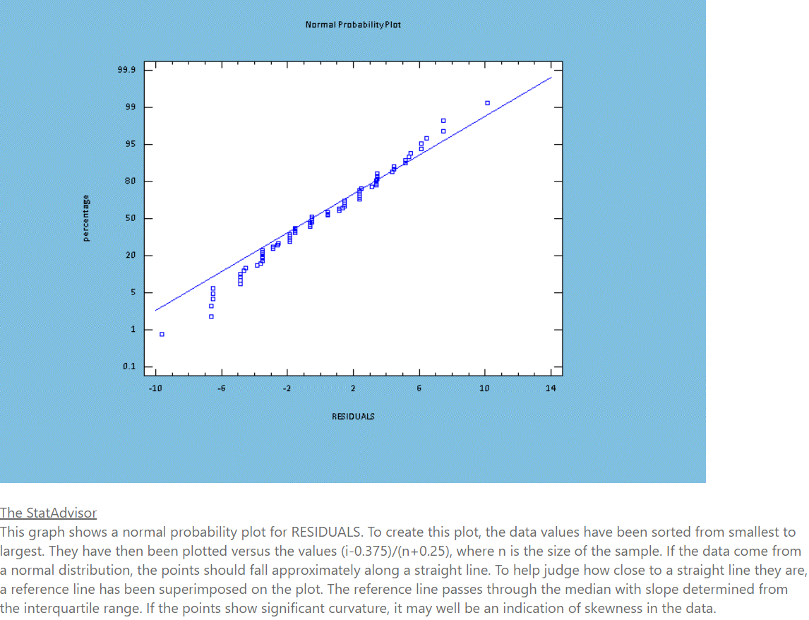
Transcribed Image Text:Normal Probability Plot
99.9
99
95
80
50
20
5.
0.1
-10
-6
-2
6
10
14
RESIDUALS
The StatAdvisor
This graph shows a normal probability plot for RESIDUALS. To create this plot, the data values have been sorted from smallest to
largest. They have then been plotted versus the values (i-0.375)/(n+0.25), where n is the size of the sample. If the data come from
a normal distribution, the points should fall approximately along a straight line. To help judge how close to a straight line they are,
a reference line has been superimposed on the plot. The reference line passes through the median with slope determined from
the interquartile range. If the points show significant curvature, it may well be an indication of skewness in the data.
Expert Solution
This question has been solved!
Explore an expertly crafted, step-by-step solution for a thorough understanding of key concepts.

Step by step
Solved in 3 steps

Knowledge Booster


Learn more about
Need a deep-dive on the concept behind this application? Look no further. Learn more about this topic, statistics and related others by exploring similar questions and additional content below.Recommended textbooks for you
MATLAB: An Introduction with Applications
Statistics
ISBN:
9781119256830
Author:
Amos Gilat
Publisher:
John Wiley & Sons Inc

Probability and Statistics for Engineering and th…
Statistics
ISBN:
9781305251809
Author:
Jay L. Devore
Publisher:
Cengage Learning

Statistics for The Behavioral Sciences (MindTap C…
Statistics
ISBN:
9781305504912
Author:
Frederick J Gravetter, Larry B. Wallnau
Publisher:
Cengage Learning
MATLAB: An Introduction with Applications
Statistics
ISBN:
9781119256830
Author:
Amos Gilat
Publisher:
John Wiley & Sons Inc
Probability and Statistics for Engineering and th…
Statistics
ISBN:
9781305251809
Author:
Jay L. Devore
Publisher:
Cengage Learning
Statistics for The Behavioral Sciences (MindTap C…
Statistics
ISBN:
9781305504912
Author:
Frederick J Gravetter, Larry B. Wallnau
Publisher:
Cengage Learning

Elementary Statistics: Picturing the World (7th E…
Statistics
ISBN:
9780134683416
Author:
Ron Larson, Betsy Farber
Publisher:
PEARSON

The Basic Practice of Statistics
Statistics
ISBN:
9781319042578
Author:
David S. Moore, William I. Notz, Michael A. Fligner
Publisher:
W. H. Freeman

Introduction to the Practice of Statistics
Statistics
ISBN:
9781319013387
Author:
David S. Moore, George P. McCabe, Bruce A. Craig
Publisher:
W. H. Freeman