stic for the model developed from the estimation data in Problem 11.2. How well is the model likely to predict? Compare this indication of predictive performance with the
stic for the model developed from the estimation data in Problem 11.2. How well is the model likely to predict? Compare this indication of predictive performance with the

Linear Algebra: A Modern Introduction
4th Edition
ISBN:9781285463247
Author:David Poole
Publisher:David Poole
Chapter7: Distance And Approximation
Section7.3: Least Squares Approximation
Problem 31EQ

Related questions
Question
Calculate the PRESS statistic for the model developed from the estimation
data in Problem 11.2. How well is the model likely to predict? Compare this
indication of predictive performance with the actual performance observed
in Problem 11.2.
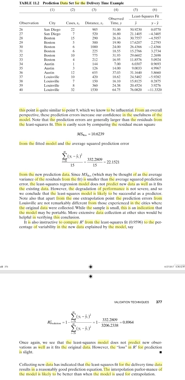
Transcribed Image Text:TABLE 11.2 Prediction Data Set for the Delivery Time Example
(1)
(2)
(3)
(4)
(5)
(6)
Least-Squares Fit
Observed
Time, y
Observation
City
Cases, x
Distance, X
y- ŷ
San Diego
San Diego
Boston
26
22
50.9230
21.1405
905
51.00
0.0770
-4.3405
-4.5957
27
520
16.80
28
15
290
26.16
30.7557
29
Boston
5
500
19.90
17.6207
2.2793
26.4366
-2.4366
3.2734
2.2698
30
Boston
1000
24.00
18,55
31.93
16.95
31
Boston
225
15.2766
32
Boston
10
775
29.6602
33
Boston
4
212
11.8576
5.0924
34
Austin
1
144
7.00
6.0307
0.9693
35
Austin
3
126
14.00
9.0033
4.9967
36
Austin
12
655
37.03
31.1640
5.8660
37
Louisville
10
420
18.62
24.5482
-5.9282
Louisville
15.8125
20.4524
38
7
150
16.10
0.2875
39
Louisville
8
360
24.38
3.9276
40
Louisville
32
1530
64.75
76.0820
-11.3320
this point is quite similar to point 9, which we know to be influential. From an overall
perspective, these prediction errors increase our confidence in the usefulness of the
model. Note that the prediction errors are generally larger than the residuals from
the least-squares fit. This is easily seen by comparing the residual mean square
MSRes = 10.6239
from the fitted model and the average squared prediction error
40
332.2809
- 22.1521
i=26
15
15
from the new prediction data. Since MSRes (which may be thought of as the average
variance of the residuals from the fit) is smaller than the average squared prediction
error, the least-squares regression model does not predict new data as well as it fits
the existing data. However, the degradation of performance is not severe, and so
we conclude that the least-squares model is likely to be successful as a predictor.
Note also that apart from the one extrapolation point the prediction errors from
Louisville are not remarkably different from thosc experienced in the citics where
the
original data were collected. While the sample is small, this is an indication that
the model may be portable. More extensive data collection at other sites would be
helpful in verifying this conclusion.
It is also instructive to compare R from the least-squares fit (0.9596) to the per-
centage of variability in the new data explained by the model, say
dd 376
vighr
6/27/2017 636:52 P
VALIDATION TECHNIQUES
377
40
332.2809
= 1
0.8964
'rediction
40
3206.2338
i=26
Once again, we see that the least-squares model does not predict new obser-
vations as well as it fits the original data. However, the "loss" in R for prediction
is slight.
Collecting new data has indicated that the least-squares fit for the delivery time data
results in a reasonably good prediction equation. The interpolation parlor-mance of
the model is likely to be better than when the model is used for extrapolation.
Expert Solution
This question has been solved!
Explore an expertly crafted, step-by-step solution for a thorough understanding of key concepts.

Step by step
Solved in 2 steps with 1 images

Recommended textbooks for you
Linear Algebra: A Modern Introduction
Algebra
ISBN:
9781285463247
Author:
David Poole
Publisher:
Cengage Learning

College Algebra
Algebra
ISBN:
9781305115545
Author:
James Stewart, Lothar Redlin, Saleem Watson
Publisher:
Cengage Learning

Big Ideas Math A Bridge To Success Algebra 1: Stu…
Algebra
ISBN:
9781680331141
Author:
HOUGHTON MIFFLIN HARCOURT
Publisher:
Houghton Mifflin Harcourt
Linear Algebra: A Modern Introduction
Algebra
ISBN:
9781285463247
Author:
David Poole
Publisher:
Cengage Learning
College Algebra
Algebra
ISBN:
9781305115545
Author:
James Stewart, Lothar Redlin, Saleem Watson
Publisher:
Cengage Learning
Big Ideas Math A Bridge To Success Algebra 1: Stu…
Algebra
ISBN:
9781680331141
Author:
HOUGHTON MIFFLIN HARCOURT
Publisher:
Houghton Mifflin Harcourt