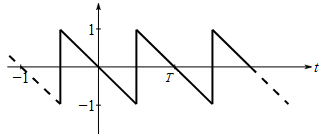
Given Information: The sawtooth wave shown as,
Formula used:
Consider f(t) is a periodic function with period T defined in the interval 0≤x≤T then the Fourier series expansion of the function is,
f(t)=a0+∑k=1∞[akcos(kω0t)+bksin(kω0t)];ω0=2πT
And the coefficients are defined by,
a0=1T∫0Tf(t)dt ; ak=2T∫0Tf(t)cos(kω0t)dt ; bk=2T∫0Tf(t)sin(kω0t)dt
Calculation:
Consider the sawtooth wave as shown in the following figure,
Therefore, the sawtooth wave is a periodic function f(t) with period T in the interval 0≤t≤T and from the graph,
f(t) is a straight line joining the points (0,0) and (T2,−1) in 0≤t≤T2
; f(t) is a straight line joining the points (T2,1) and (T,0) in T2≤t≤T.
Therefore, the sawtooth wave,
f(t)={−2Tt,0≤t≤T22−2Tt,T2≤t≤T
Therefore, the Fourier series expansion of the function f(t) is,
f(t)=a0+∑k=1∞[akcos(kω0t)+bksin(kω0t)] with ω0=2πT.
Here, the coefficients are defined by,
a0=1T∫0Tf(t)dt ; ak=2T∫0Tf(t)cos(2kπTt)dt ; bk=2T∫0Tf(t)sin(2kπTt)dt
Now, find ak.
ak=2T∫0Tf(t)cos(2kπTt)dt=2T∫0T2(−2Tt)cos(2kπTt)dt+2T∫T2T(2−2Tt)cos(2kπTt)dt=−4T2∫0T2tcos(2kπTt)dt+4T∫T2Tcos(2kπTt)dt−4T2∫T2Ttcos(2kπTt)dt
Consider,
I=∫tcos(2kπTt)dt=t∫cos(2kπTt)dt−∫{ddt(t)∫cos(2kπTt)dt}dt=tT2kπsin(2kπTt)−∫T2kπsin(2kπTt)dt=Tt2kπsin(2kπTt)+T24k2π2cos(2kπTt)
Thus,
∫0T2tcos(2kπTt)dt=[Tt2kπsin(2kπTt)+T24k2π2cos(2kπTt)]0T2=T2kπT2sin(2kπTT2)+T24k2π2cos(2kπTT2)−T24k2π2cos(0)=T24kπsin(kπ)+T24k2π2cos(kπ)−T24k2π2=T24k2π2(−1)k−T24k2π2
∫T2Tcos(2kπTt)dt=T2kπsin(2kπTt)|T2T=T2kπ{sin(2kπ)−sin(kπ)}=0
∫T2Ttcos(2kπTt)dt=[Tt2kπsin(2kπTt)+T24k2π2cos(2kπTt)]T2T=T22kπsin(2kπ)+T24k2π2cos(2kπ)−T24kπsin(kπ)−T24k2π2cos(kπ)=T24k2π2−T24k2π2(−1)k
Therefore,
ak=−4T2[T24k2π2(−1)k−T24k2π2]+4T×0−4T2[T24k2π2−T24k2π2(−1)k]=−1k2π2(−1)k+1k2π2−1k2π2+1k2π2(−1)k=0
Now, find bk.
bk=2T∫0Tf(t)sin(2kπTt)dt=2T∫0T2(−2Tt)sin(2kπTt)dt+2T∫T2T(2−2Tt)sin(2kπTt)dt=−4T2∫0T2tsin(2kπTt)dt+4T∫T2Tsin(2kπTt)dt−4T2∫T2Ttsin(2kπTt)dt
Consider,
I=∫tsin(2kπTt)dt=t∫sin(2kπTt)dt−∫{ddt(t)∫sin(2kπTt)dt}dt=−tT2kπcos(2kπTt)+∫T2kπcos(2kπTt)dt=−Tt2kπcos(2kπTt)+T24k2π2sin(2kπTt)
Thus,
∫0T2tsin(2kπTt)dt=[−Tt2kπcos(2kπTt)+T24k2π2sin(2kπTt)]0T2=−T24kπcos(kπ)+T24k2π2sin(kπ)=−T24kπ(−1)k
∫T2Tsin(2kπTt)dt=−T2kπcos(2kπTt)|T2T=−T2kπcos(2kπ)+T2kπcos(kπ)=−T2kπ+T2kπ(−1)k
Further,
∫T2Ttsin(2kπTt)dt=[−Tt2kπcos(2kπTt)+T24k2π2sin(2kπTt)]T2T=−T22kπcos(2kπ)+T24k2π2sin(2kπ)+T24kπcos(kπ)−T24k2π2sin(kπ)=−T22kπ+T24kπ(−1)k
Therefore,
bk=−4T2[−T24kπ(−1)k]+4T[−T2kπ+T2kπ(−1)k]−4T2[−T22kπ+T24kπ(−1)k]=1kπ(−1)k−2kπ+2kπ(−1)k+2kπ−1kπ(−1)k=2kπ(−1)k
Therefore, the coefficients of the Fourier series expansions are,
a0=0, ak=0, bk=2kπ(−1)k
Therefore, the Fourier series expansion defines ω0=2πT, f(t)=∑k=1∞[2kπ(−1)ksin(kω0t)]=2π∑k=1∞[(−1)kksin(kω0t)]
Hence, f(t)=2π[−sin(ω0t)+12sin(2ω0t)−13sin(3ω0t)+...]
Graph:
To plot the given sawtooth curve and the approximated Fourier series consider the period, T=1.
Therefore, the periodic sawtooth curve is expressed as,
f(t)={−2t,0≤t≤122−2t,12≤t≤1
And, the corresponding Fourier series is,
f(t)=2π[−sin(ω0t)+12sin(2ω0t)−13sin(3ω0t)+...],ω0=2π
Hence, f(t)=−2πsin(2πt)+1πsin(4πt)−23πsin(6πt)+...
Use the following MATLAB code to plot the first three terms along with the summation.
function Code_97924_19_4P()
% enter the time period
T = 1;
t1 = 0: 0.0001: T/2;
t2 = T/2: 0.0001: T;
% define the function
f1 = @(t) -(2/T)*t;
f2 = @(t) 2-(2/T)*t;
t = [t1, t2];
f = [f1(t1), f2(t2)];
w0 = 2*pi/T;
% define the first three terms in the series
Term1 = @(t) -(2/pi)*sin(w0*t);
Term2 = @(t) (1/pi)*sin(2*w0*t);
Term3 = @(t) -(2/(3*pi))*sin(3*w0*t);
ff = @(t) Term1(t) + Term2(t) + Term3(t);
% plot the results
figure(); hold on
plot(t,f,'–k','Linewidth',2);
plot(t, Term1(t),'-.m','Linewidth',2);
plot(t, Term2(t),'-.r','Linewidth',2);
plot(t, Term3(t),'-.g','Linewidth',2);
plot(t, ff(t),'b','Linewidth',2);
% define the graphical properties
ylim([-2 2]); grid on
legend('Original','1^{st} Term','2^{nd} Term','3^{rd} Term','Sum')
set(gca,'XTick',[0 T/4 T/2 3*T/4 T]);
set(gca,'XTickLabel',{'0' 'T/4' 'T/2' '3T/4' 'T'});
set(gca,'Fontname','Times New Roman','FontSize',12);
end
Execute the above code to obtain the plot as,
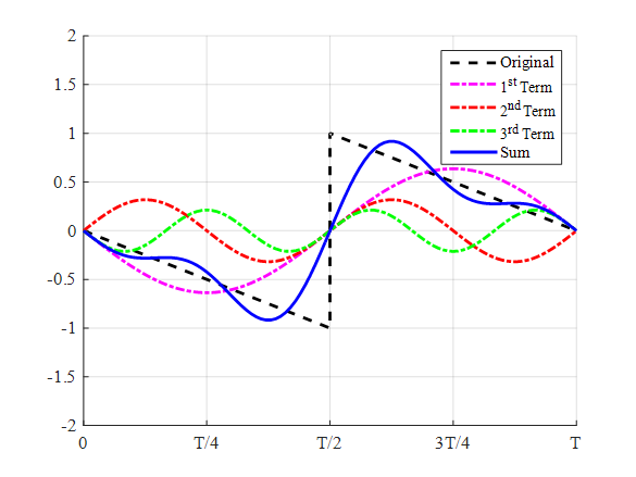
Interpretation: The above plot shows the comparison between the variation in the first three terms of the series along with the variation in summation.


 Trigonometry (MindTap Course List)TrigonometryISBN:9781305652224Author:Charles P. McKeague, Mark D. TurnerPublisher:Cengage Learning
 Algebra & Trigonometry with Analytic GeometryAlgebraISBN:9781133382119Author:SwokowskiPublisher:Cengage
 Trigonometry (MindTap Course List)TrigonometryISBN:9781337278461Author:Ron LarsonPublisher:Cengage Learning