
Videos
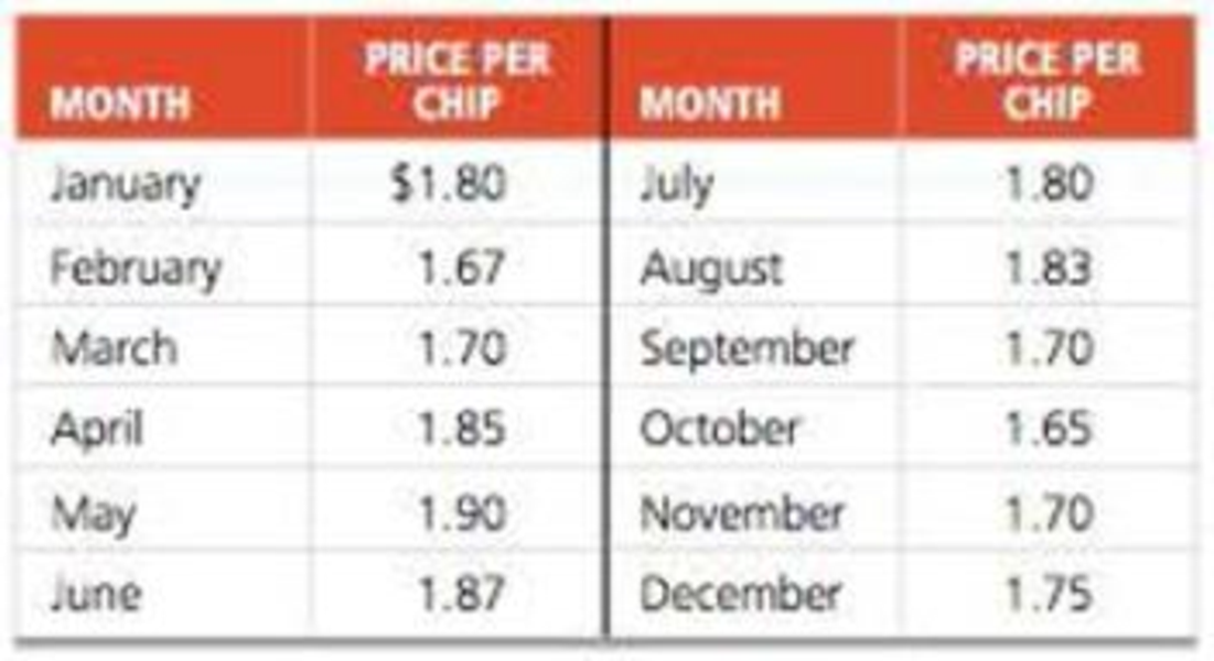
Lenovo uses the ZX-81 chip in some of its laptop computers. The prices for the chip during the past 12 months were as follows:
a) Use a 2-month moving average on all the data and plot the averages and the prices.
b) Use a 3-month moving average and add the 3-month plot to the graph created in part (a).
c) Which is better (using the mean absolute deviation): the 2-month average or the 3-month average?
d) Compute the
a)
To determine:Plot and graphically represent the averages and the prices using 2-month moving average.
Introduction: Forecasting is used to predict future changes or a demand pattern. It involves different approaches and varies with different time periods. Moving average, weighted moving average and exponential smoothing are the time series methods of forecasting which uses past data to forecast the future.
Answer to Problem 9P
By using 2-month moving average, the averages and the prices are plotted.
Explanation of Solution
Given information:
| Month | Price Per Chip |
| January | 1.80 |
| February | 1.67 |
| March | 1.70 |
| April | 1.85 |
| May | 1.90 |
| June | 1.87 |
| July | 1.80 |
| August | 1.83 |
| September | 1.70 |
| October | 1.65 |
| November | 1.70 |
| December | 1.75 |
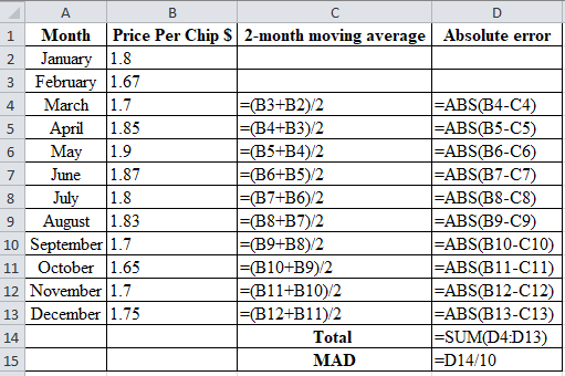
Formula to calculate the forecasted demand
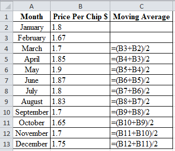
| Month | Price Per Chip $ | Moving Average |
| January | 1.8 | |
| February | 1.67 | |
| March | 1.7 | 1.735 |
| April | 1.85 | 1.685 |
| May | 1.9 | 1.775 |
| June | 1.87 | 1.875 |
| July | 1.8 | 1.885 |
| August | 1.83 | 1.835 |
| September | 1.7 | 1.815 |
| October | 1.65 | 1.765 |
| November | 1.7 | 1.675 |
| December | 1.75 | 1.675 |
Table 1
Excel worksheet:
Calculation of the forecast for March:
To calculate the forecast for March, divide the summation of the values of January and February by 2. The corresponding value 1.735 is the forecast for March. The 2-month moving average for the month of March is 1.735.
Calculation of the forecast for April:
To calculate the forecast for April, divide the summation of the values of February and March by 2. The corresponding value 1.685 is the forecast for April. The 2-month moving average for the month of April is 1.685.
Calculation of the forecast for May:
To calculate the forecast for May, divide the summation of the values of March and April by 2. The corresponding value 1.775 is the forecast for May. The 2-month moving average for the month of May is 1.775.
Calculation of the forecast for June:
To calculate the forecast for June, divide the summation of the values of April and May by 2. The corresponding value 1.875 is the forecast for June. The 2-month moving average for the month of June is 1.875.
Calculation of the forecast for July:
To calculate the forecast for July, divide the summation of the values of May and June by 2. The corresponding value 1.885 is the forecast for July. The 2-month moving average for the month of July is 1.885
Calculation of the forecast for August:
To calculate the forecast for August, divide the summation of the values of June and July by 2. The corresponding value 1.835 is the forecast for August. The 2-month moving average for the month of August is 1.685.
Calculation of the forecast for September:
To calculate the forecast for September, divide the summation of the values of July and August by 2. The corresponding value 1.815 is the forecast for September. The 2-month moving average for the month of September is 1.815.
Calculation of the forecast for October:
To calculate the forecast for October, divide the summation of the values of August and September by 2. The corresponding value 1.765 is the forecast for October. The 2-month moving average for the month of October is 1.765.
Calculation of the forecast for November:
To calculate the forecast for November, divide the summation of the values of September and October by 2. The corresponding value 1.675 is the forecast for November. The 2-month moving average for the month of November is 1.675.
Calculation of the forecast for December:
To calculate the forecast for December, divide the summation of the values of October and November by 2. The corresponding value 1.675 is the forecast for December. The 2-month moving average for the month of December is 1.675.
Graph:
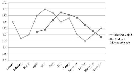
The data for 2-month moving average is obtained from Table 1. Graph is plotted with price per chip, and 2-month moving average.
Hence, the graphical representation of the averages and the prices are plotted using 2-month moving average.
b)
To determine:Plot and graphically represent the averages and the prices using 3-month moving average.
Answer to Problem 9P
By using 3-month moving average, the averages and the prices are plotted.
Explanation of Solution
Given information:
| Month | Price Per Chip |
| January | 1.80 |
| February | 1.67 |
| March | 1.70 |
| April | 1.85 |
| May | 1.90 |
| June | 1.87 |
| July | 1.80 |
| August | 1.83 |
| September | 1.70 |
| October | 1.65 |
| November | 1.70 |
| December | 1.75 |
Formula to calculate the forecasted demand:
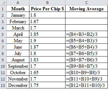
| Month | Price Per Chip $ | Moving Average |
| January | 1.8 | |
| February | 1.67 | |
| March | 1.7 | |
| April | 1.85 | 1.723 |
| May | 1.9 | 1.740 |
| June | 1.87 | 1.817 |
| July | 1.8 | 1.873 |
| August | 1.83 | 1.857 |
| September | 1.7 | 1.833 |
| October | 1.65 | 1.777 |
| November | 1.7 | 1.727 |
| December | 1.75 | 1.683 |
Table 2
Excel worksheet:
Calculation of the forecast for April:
To calculate the forecast for April, divide the summation of the values of January, February and March by 3. The corresponding value 1.732 is the forecast for April. Therefore, 3-month moving average for the month of April is 1.723.
Calculation of the forecast for May:
To calculate the forecast for May, divide the summation of the values of February, March and April by 3. The corresponding value 1.740 is the forecast for May. Therefore, 3-month moving average for the month of May is 1.740.
Calculation of the forecast for June:
To calculate the forecast for June, divide the summation of the values of March, April and May by 3. The corresponding value 1.817 is the forecast for June. Therefore, 3-month moving average for the month of June is 1.817.
Calculation of the forecast for July:
To calculate the forecast for July, divide the summation of the values of April, May and June by 3. The corresponding value 1.873 is the forecast for July. Therefore, 3-month moving average for the month of July is 1.873.
Calculation of the forecast for August:
To calculate the forecast for August, divide the summation of the values of May, June and July by 3. The corresponding value 1.873 is the forecast for August. Therefore, 3-month moving average for the month of August is 1.873.
Calculation of the forecast for September:
To calculate the forecast for September, divide the summation of the values of June, July and August by 3. The corresponding value 1.833 is the forecast for September. Therefore, 3-month moving average for the month of June is 1.833.
Calculation of the forecast for October:
To calculate the forecast for October, divide the summation of the values of July, August and September by 3. The corresponding value 1.777 is the forecast for October. Therefore, 3-month moving average for the month of June is 1.777.
Calculation of the forecast for November:
To calculate the forecast for November, divide the summation of the values of August, September and October by 3. The corresponding value 1.727 is the forecast for November. Therefore, 3-month moving average for the month of November is 1.727.
Calculation of the forecast for December:
To calculate the forecast for December, divide the summation of the values of September, October and November by 3. The corresponding value 1.683 is the forecast for December. Therefore, 3-month moving average for the month of December is 1.683.
Graph:
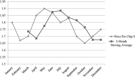
The data for 3-month moving average is obtained from Table 2. Graph is plotted with price per chip, and 3-month moving average.
Hence, the graphical representation of the averages and the prices are plotted using 3-month moving average.
c)
To determine:Compute the Mean Absolute Deviation (MAD) using 2-month moving average and 3-month moving average and from the results, infer the superior method.
Answer to Problem 9P
MAD from 2-month moving average and 3-month moving average are 0.075 & 0.079 (refer to equations (1) & (2)). Because of less deviation of error, MAD from a 2-month moving average is superior over a 3-month moving average.
Explanation of Solution
Given information:
| Month | Price Per Chip |
| January | 1.80 |
| February | 1.67 |
| March | 1.70 |
| April | 1.85 |
| May | 1.90 |
| June | 1.87 |
| July | 1.80 |
| August | 1.83 |
| September | 1.70 |
| October | 1.65 |
| November | 1.70 |
| December | 1.75 |
Formula to calculate MAD:
Calculation of MAD using 2-month moving average:
Table 1 provides the calculation of forecast using 2-month moving average.
| Month | Price Per Chip $ | 2-month moving average | Absolute error |
| January | 1.8 | ||
| February | 1.67 | ||
| March | 1.7 | 1.735 | 0.035 |
| April | 1.85 | 1.685 | 0.165 |
| May | 1.9 | 1.775 | 0.125 |
| June | 1.87 | 1.875 | 0.005 |
| July | 1.8 | 1.885 | 0.085 |
| August | 1.83 | 1.835 | 0.005 |
| September | 1.7 | 1.815 | 0.115 |
| October | 1.65 | 1.765 | 0.115 |
| November | 1.7 | 1.675 | 0.025 |
| December | 1.75 | 1.675 | 0.075 |
| Total | 0.75 | ||
| MAD | 0.075 |
Excel worksheet:
Calculation of the absolute error for March:
Absolute Error of March is the modulus of the difference between 1.7 and 1.735, which corresponds to 0.035. Therefore Absolute Error for March is 0.035.
Calculation of the absolute error for April:
Absolute Error of April is the modulus of the difference between 1.85 and 1.685, which corresponds to 0.165. Therefore Absolute Error for April is 0.165.
Calculation of the absolute error for May:
Absolute Error of May is the modulus of the difference between 1.9 and 1.775, which corresponds to 0.125. Therefore Absolute Error for May is 0.125.
Calculation of the absolute error for June:
Absolute Error of June is the modulus of the difference between 1.87 and 1.875, which corresponds to 0.005. Therefore Absolute Error for June is 0.005.
Calculation of the absolute error for July:
Absolute Error of July is the modulus of the difference between 1.8 and 1.885, which corresponds to 0.085. Therefore Absolute Error for July is 0.085.
Calculation of the absolute error for August:
Absolute Error of August is the modulus of the difference between 1.83 and 1.835, which corresponds to 0.005. Therefore Absolute Error for August is 0.005.
Calculation of the absolute error for September:
Absolute Error of September is the modulus of the difference between 1.7 and 1.815, which corresponds to 0.115. Therefore Absolute Error for September is 0.115.
Calculation of the absolute error for October:
Absolute Error of October is the modulus of the difference between 1.65 and 1.765, which corresponds to 0.115. Therefore Absolute Error for October is 0.115.
Calculation of the absolute error for November:
Absolute Error of November is the modulus of the difference between 1.7 and 1.675, which corresponds to 0.025. Therefore Absolute Error for November is 0.025.
Calculation of the absolute error for December:
Absolute Error of December is the modulus of the difference between 1.75 and 1.675, which corresponds to 0.075. Therefore Absolute Error for December is 0.075.
Calculation of MAD using 2-month moving average:
Mean Absolute Deviation is obtained by dividing the summation of absolute values by the number of years. Absolute error is obtained by taking modulus for the difference between Actual and forecasted values.
Substitute the summation value of absolute error for 10 years i.e. 0.75 is divided by number of years i.e. 10 yields MAD of 0.075
The Mean Absolute Deviation using 2-month moving average is 0.075
Calculation of MAD using 3-month moving average
Table 2 provides the value of 3-month moving average
| Month | Price Per Chip $ | 3-month Moving Average | Absolute error |
| January | 1.8 | ||
| February | 1.67 | ||
| March | 1.7 | ||
| April | 1.85 | 1.723 | 0.127 |
| May | 1.9 | 1.740 | 0.160 |
| June | 1.87 | 1.817 | 0.053 |
| July | 1.8 | 1.873 | 0.073 |
| August | 1.83 | 1.857 | 0.027 |
| September | 1.7 | 1.833 | 0.133 |
| October | 1.65 | 1.777 | 0.127 |
| November | 1.7 | 1.727 | 0.027 |
| December | 1.75 | 1.683 | 0.067 |
| Total | 0.793 | ||
| MAD | 0.079 |
Excel worksheet:
Calculation of the Absolute Error for April:
Absolute Error of April is the modulus of the difference between 1.85 and 1.723, which corresponds to 0.127. Absolute Error for April is 0.127
Calculation of the Absolute Error for May:
Absolute Error of May is the modulus of the difference between 1.9 and 1.740, which corresponds to 0.160. Therefore Absolute Error for May is 0.160
Calculation of the Absolute Error for June:
Absolute Error of June is the modulus of the difference between 1.87 and 1.817, which corresponds to 0.053. Therefore Absolute Error for June is 0.053
Calculation of the Absolute Error for July:
Absolute Error of July is the modulus of the difference between 1.8 and 1.873, which corresponds to 0.073. Absolute Error for July is 0.073.
Calculation of the Absolute Error for August:
Absolute Error of August is the modulus of the difference between 1.83 and 1.857, which corresponds to 0.027. Therefore, Absolute Error for August is 0.027.
Calculation of the Absolute Error for September:
Absolute Error of September is the modulus of the difference between 1.7 and 1.833, which corresponds to 0.133. Therefore Absolute Error for September is 0.133.
Calculation of the Absolute Error for October:
Absolute Error of October is the modulus of the difference between 1.65 and 1.777, which corresponds to 0.127. Therefore Absolute Error for October is 0.127.
Calculation of the Absolute Error for November:
Absolute Error of November is the modulus of the difference between 1.7 and 1.727, which corresponds to 0.027. Therefore Absolute Error for November is 0.027
Calculation of the Absolute Error for December:
Absolute Error of December is the modulus of the difference between 1.75 and 1.683, which corresponds to 0.067. Therefore Absolute Error for December is 0.067
Calculation of MAD using 3-month moving average:
Substitute the summation value of absolute error for 10 years i.e. 0.793 is divided by number of years i.e. 9 yields MAD of 0.079. Mean Absolute Deviation using 3-month moving average is 0.079
Hence, the Mean Absolute Deviation from the 2-month moving average is 0.075 (refer to equation (1)) and from the 3-month moving average is 0.079 (refer to equation (2)). Due to less deviation of error, the MAD from the 2-month moving average is superior to that of the 3-month moving average.
d)
To determine: Decide the best method by computing Mean Absolute Duration using exponential smoothing with α = 0.1, α = 0.3 and α = 0.5
Answer to Problem 9P
The Mean Absolute Deviation using exponential smoothing using α = 0.1 is 0.071, (refer to equation 3), α = 0.3 is 0.070 (refer to equation 4) and α = 0.5 is 0.066 (refer to equation 5). MAD using α = 0.5 is the best method since the MAD is minimum.
Explanation of Solution
Given information:
| Month | Price Per Chip |
| January | 1.80 |
| February | 1.67 |
| March | 1.70 |
| April | 1.85 |
| May | 1.90 |
| June | 1.87 |
| July | 1.80 |
| August | 1.83 |
| September | 1.70 |
| October | 1.65 |
| November | 1.70 |
| December | 1.75 |
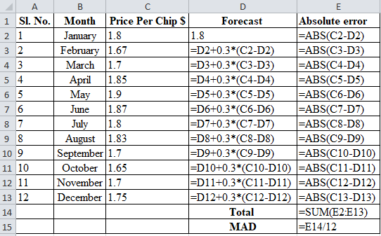
The initial forecast for the month of January is $1.80
Formula to calculate the forecasted demand
Where,
Calculation of MAD using exponential smoothing with smoothing constant α = 0.1
| Sl. No. | Month | Price Per Chip $ | Forecast | Absolute error |
| 1 | January | 1.8 | 1.8 | 0 |
| 2 | February | 1.67 | 1.8 | 0.130 |
| 3 | March | 1.7 | 1.787 | 0.087 |
| 4 | April | 1.85 | 1.778 | 0.072 |
| 5 | May | 1.9 | 1.785 | 0.115 |
| 6 | June | 1.87 | 1.797 | 0.073 |
| 7 | July | 1.8 | 1.804 | 0.004 |
| 8 | August | 1.83 | 1.804 | 0.026 |
| 9 | September | 1.7 | 1.806 | 0.106 |
| 10 | October | 1.65 | 1.796 | 0.146 |
| 11 | November | 1.7 | 1.781 | 0.081 |
| 12 | December | 1.75 | 1.773 | 0.023 |
| Total | 0.8632 | |||
| MAD | 0.0719 |
Excel worksheet:
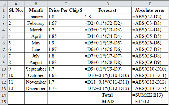
Calculation of absolute error for January:
Absolute Error of January is the modulus of the difference between 1.8 and 1.8, which corresponds to 0. Therefore Absolute Error for January is 0
Calculation of the forecast & absolute error for February:
To calculate forecast for February, substitute the value of forecast of January, smoothing constant and difference of actual and forecasted demand in the above formula. The result of forecast for February is 1.8
Absolute Error of February is the modulus of the difference between 1.67 and 1.8, which corresponds to 0.130 Therefore Absolute Error for February, is 0.130
Forecast and Absolute error for February is 1.8 & 0.130
Calculation of the forecast & absolute error for March:
To calculate forecast for March, substitute the value of forecast of February, smoothing constant and difference of actual and forecasted demand in the above formula. The result of forecast for March is 1.787
Absolute Error of March is the modulus of the difference between 1.7 and 1.787, which corresponds to 0.087 Therefore Absolute Error for March, is 0.087
Forecast and Absolute error for March is 1.787 & 0.087
Calculation of the forecast & absolute error for April:
To calculate forecast for April, substitute the value of forecast of March, smoothing constant and difference of actual and forecasted demand in the above formula. The result of forecast for April is 1.778.
Absolute Error of April is the modulus of the difference between 1.85 and 1.778, which corresponds to 0.072. Therefore Absolute Error for April is 0.087.
Forecast and Absolute error for April is 1.778 & 0.072.
Calculation of the forecast & absolute error for May:
To calculate forecast for May, substitute the value of forecast of April, smoothing constant and difference of actual and forecasted demand in the above formula. The result of forecast for May is 1.785
Absolute Error of May is the modulus of the difference between 1.9 and 1.785, which corresponds to 0.115. Therefore Absolute Error for May is 0.115
Forecast and Absolute error for May is 1.785 & 0.115
Calculation of the forecast & absolute error for June:
To calculate forecast for June, substitute the value of forecast of May, smoothing constant and difference of actual and forecasted demand in the above formula. The result of forecast for June is 1.797.
Absolute Error of June is the modulus of the difference between 1.87 and 1.797, which corresponds to 0.073. Therefore Absolute Error for June is 0.073.
Forecast and Absolute error for June is 1.797 & 0.073.
Calculation of the forecast & absolute error for July:
To calculate forecast for July, substitute the value of forecast of June, smoothing constant and difference of actual and forecasted demand in the above formula. The result of forecast for July is 1.804
Absolute Error of July is the modulus of the difference between 1.8 and 1.804, which corresponds to 0.004. Therefore Absolute Error for July is 0.004
Forecast and Absolute error for July is 1.804 & 0.004
Calculation of the forecast & absolute error for August:
To calculate forecast for August, substitute the value of forecast of July, smoothing constant and difference of actual and forecasted demand in the above formula. The result of forecast for August is 1.804
Absolute Error of August is the modulus of the difference between 1.83 and 1.804, which corresponds to 0.026. Therefore Absolute Error for July is 0.026
Forecast and Absolute error for August is 1.804 & 0.026
Calculation of the forecast & absolute error for September:
To calculate forecast for September, substitute the value of forecast of August, smoothing constant and difference of actual and forecasted demand in the above formula. The result of forecast for September is 1.806
Absolute Error of September is the modulus of the difference between 1.7 and 1.806, which corresponds to 0.106 Therefore Absolute Error for September, is 0.106
Forecast and Absolute error for September is 1.806 & 0.106
Calculation of the forecast & absolute error for October:
To calculate forecast for October, substitute the value of forecast of September, smoothing constant and difference of actual and forecasted demand in the above formula. The result of forecast for October is 1.796
Absolute Error of October is the modulus of the difference between 1.65 and 1.796, which corresponds to 0.146 Therefore Absolute Error for October, is 0.146
Forecast and Absolute error for October is 1.796 & 0.146
Calculation of the forecast & absolute error for November:
To calculate forecast for November, substitute the value of forecast of October, smoothing constant and difference of actual and forecasted demand in the above formula. The result of forecast for November is 1.781.
Absolute Error of November is the modulus of the difference between 1.7 and 1.781, which corresponds to 0.081 Therefore Absolute Error for November, is 0.081.
Forecast and Absolute error for November is 1.781 & 0.081.
Calculation of the forecast & absolute error for December:
To calculate forecast for December, substitute the value of forecast of November, smoothing constant and difference of actual and forecasted demand in the above formula. The result of forecast for December is 1.773.
Absolute Error of December is the modulus of the difference between 1.75 and 1.773, which corresponds to 0.023. Therefore Absolute Error for December is 0.023.
Forecast and Absolute error for December is 1.773 & 0.023.
Calculation of MAD:
Upon substitution of summation value of absolute error for 12 years i.e. 0.8623 is divided by number of years i.e. 12 yields MAD of 0.0719
Mean Absolute Deviation using exponential smoothing with smoothing constant α = 0.1 is 0.0719
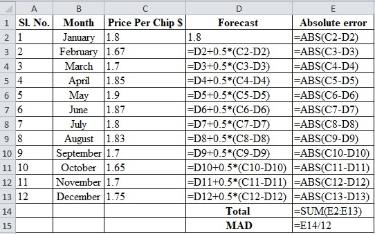
Calculation of MAD using exponential smoothing with smoothing constant α = 0.3
| Sl. No. | Month | Price Per Chip $ | Forecast | Absolute error |
| 1 | January | 1.8 | 1.8 | 0 |
| 2 | February | 1.67 | 1.800 | 0.130 |
| 3 | March | 1.7 | 1.761 | 0.061 |
| 4 | April | 1.85 | 1.743 | 0.107 |
| 5 | May | 1.9 | 1.775 | 0.125 |
| 6 | June | 1.87 | 1.812 | 0.058 |
| 7 | July | 1.8 | 1.830 | 0.030 |
| 8 | August | 1.83 | 1.821 | 0.009 |
| 9 | September | 1.7 | 1.824 | 0.124 |
| 10 | October | 1.65 | 1.786 | 0.136 |
| 11 | November | 1.7 | 1.746 | 0.046 |
| 12 | December | 1.75 | 1.732 | 0.018 |
| Total | 0.844 | |||
| MAD | 0.070 |
Excel worksheet:
Calculation of the absolute error for January:
Absolute Error of January is the modulus of the difference between 1.8 and 1.8, which corresponds to 0. Therefore Absolute Error for January is 0
Calculation of the forecast & absolute error for February:
To calculate forecast for February, substitute the value of forecast of January, smoothing constant and difference of actual and forecasted demand in the above formula. The result of forecast for February is 1.8.
Absolute Error of February is the modulus of the difference between 1.67 and 1.8, which corresponds to 0.130 Therefore Absolute Error for February, is 0.130.
Forecast and Absolute error for February is 1.800 & 0.130.
Calculation of the forecast & absolute error for March:
To calculate forecast for March, substitute the value of forecast of February, smoothing constant and difference of actual and forecasted demand in the above formula. The result of forecast for March is 1.761.
Absolute Error of March is the modulus of the difference between 1.7 and 1.761, which corresponds to 0.061 Therefore Absolute Error for March, is 0.061.
Forecast and Absolute error for March is 1.761 & 0.061.
Calculation of the forecast & absolute error for April:
To calculate forecast for April, substitute the value of forecast of March, smoothing constant and difference of actual and forecasted demand in the above formula. The result of forecast for April is 1.743.
Absolute Error of April is the modulus of the difference between 1.85 and 1.743, which corresponds to 0.107. Therefore Absolute Error for April is 0.107.
Forecast and Absolute error for April is 1.743 & 0.107.
Calculation of the forecast & absolute error for May:
To calculate forecast for May, substitute the value of forecast of April, smoothing constant and difference of actual and forecasted demand in the above formula. The result of forecast for May is 1.775.
Absolute Error of May is the modulus of the difference between 1.9 and 1.775, which corresponds to 0.125. Therefore Absolute Error for May is 0.125.
Forecast and Absolute error for May is 1.775 & 0.125.
Calculation of the forecast & absolute error for June:
To calculate forecast for June, substitute the value of forecast of May, smoothing constant and difference of actual and forecasted demand in the above formula. The result of forecast for June is 1.812.
Absolute Error of June is the modulus of the difference between 1.87 and 1.812, which corresponds to 0.058. Therefore Absolute Error for June is 0.058.
Forecast and Absolute error for June is 1.812 & 0.058.
Calculation of the forecast & absolute error for July:
To calculate forecast for July, substitute the value of forecast of June, smoothing constant and difference of actual and forecasted demand in the above formula. The result of forecast for July is 1.830.
Absolute Error of July is the modulus of the difference between 1.8 and 1.830, which corresponds to 0.030. Therefore Absolute Error for July is 0.030.
Forecast and Absolute error for July is 1.830 & 0.030.
Calculation of the forecast & absolute error for August:
To calculate forecast for August, substitute the value of forecast of July, smoothing constant and difference of actual and forecasted demand in the above formula. The result of forecast for August is 1.821.
Absolute Error of August is the modulus of the difference between 1.83 and 1.821, which corresponds to 0.009. Therefore Absolute Error for July is 0.009.
Forecast and Absolute error for August is 1.821 & 0.009.
Calculation of the forecast & absolute error for September:
To calculate forecast for September, substitute the value of forecast of August, smoothing constant and difference of actual and forecasted demand in the above formula. The result of forecast for September is 1.824.
Absolute Error of September is the modulus of the difference between 1.7 and 1.824, which corresponds to 0.124 Therefore Absolute Error for September, is 0.124.
Forecast and Absolute error for September is 1.824 & 0.124.
Calculation of the forecast & absolute error for October:
To calculate forecast for October, substitute the value of forecast of September, smoothing constant and difference of actual and forecasted demand in the above formula. The result of forecast for October is 1.786.
Absolute Error of October is the modulus of the difference between 1.65 and 1.786, which corresponds to 0.146 Therefore Absolute Error for October, is 0.136.
Forecast and Absolute error for October is 1.786 & 0.136.
Calculation of the forecast & absolute error for November:
To calculate forecast for November, substitute the value of forecast of October, smoothing constant and difference of actual and forecasted demand in the above formula. The result of forecast for November is 1.746.
Absolute Error of November is the modulus of the difference between 1.7 and 1.746, which corresponds to 0.046 Therefore Absolute Error for November, is 0.046.
Forecast and Absolute error for November is 1.746 & 0.046.
Calculation of the forecast & absolute error for December:
To calculate forecast for December, substitute the value of forecast of November, smoothing constant and difference of actual and forecasted demand in the above formula. The result of forecast for December is 1.732.
Absolute Error of December is the modulus of the difference between 1.75 and 1.773, which corresponds to 0.018. Therefore Absolute Error for December is 0.018.
Forecast and Absolute error for December is 1.732 & 0.018.
Calculation of the Mean Absolute Deviation:
Upon substitution of summation value of absolute error for 12 years i.e. 0.844 is divided by number of years i.e. 12 yields MAD of 0.070.
Mean Absolute Deviation using exponential smoothing with smoothing constant α = 0.3 is 0.070
Calculation of MAD using exponential smoothing with smoothing constant α = 0.5
| Sl. No. | Month | Price Per Chip $ | Forecast | Absolute error |
| 1 | January | 1.8 | 1.8 | 0 |
| 2 | February | 1.67 | 1.800 | 0.130 |
| 3 | March | 1.7 | 1.735 | 0.035 |
| 4 | April | 1.85 | 1.718 | 0.133 |
| 5 | May | 1.9 | 1.784 | 0.116 |
| 6 | June | 1.87 | 1.842 | 0.028 |
| 7 | July | 1.8 | 1.856 | 0.056 |
| 8 | August | 1.83 | 1.828 | 0.002 |
| 9 | September | 1.7 | 1.829 | 0.129 |
| 10 | October | 1.65 | 1.764 | 0.114 |
| 11 | November | 1.7 | 1.707 | 0.007 |
| 12 | December | 1.75 | 1.704 | 0.046 |
| Total | 0.797 | |||
| MAD | 0.066 |
Excel worksheet:
Calculation of the absolute error for January:
Absolute Error of January is the modulus of the difference between 1.8 and 1.8, which corresponds to 0. Therefore Absolute Error for January is 0
Absolute Error for January is 0
Calculation of the forecast & absolute error for February:
To calculate forecast for February, substitute the value of forecast of January, smoothing constant and difference of actual and forecasted demand in the above formula. The result of forecast for February is 1.8
Absolute Error of February is the modulus of the difference between 1.67 and 1.8, which corresponds to 0.130 Therefore Absolute Error for February, is 0.130
Forecast and Absolute error for February is 1.8 & 0.130
Calculation of the forecast & absolute error for March:
To calculate forecast for March, substitute the value of forecast of February, smoothing constant and difference of actual and forecasted demand in the above formula. The result of forecast for March is 1.735
Absolute Error of March is the modulus of the difference between 1.7 and 1.735, which corresponds to 0.035 Therefore Absolute Error for March, is 0.035
Forecast and Absolute error for March is 1.735 & 0.035
Calculation of the forecast & absolute error for April:
To calculate forecast for April, substitute the value of forecast of March, smoothing constant and difference of actual and forecasted demand in the above formula. The result of forecast for April is 1.718
Absolute Error of April is the modulus of the difference between 1.85 and 1.718, which corresponds to 0.133. Therefore Absolute Error for April is 0.133
Forecast and Absolute error for April is 1.718 & 0.133
Calculation of the forecast & absolute error for May:
To calculate forecast for May, substitute the value of forecast of April, smoothing constant and difference of actual and forecasted demand in the above formula. The result of forecast for May is 1.784
Absolute Error of May is the modulus of the difference between 1.9 and 1.784, which corresponds to 0.116. Therefore Absolute Error for May is 0.116
Forecast and Absolute error for May is 1.784 & 0.116
Calculation of the forecast & absolute error for June:
To calculate forecast for June, substitute the value of forecast of May, smoothing constant and difference of actual and forecasted demand in the above formula. The result of forecast for June is 1.842.
Absolute Error of June is the modulus of the difference between 1.87 and 1.842, which corresponds to 0.028. Therefore Absolute Error for June is 0.028.
Forecast and Absolute error for June is 1.842 & 0.028.
Calculation of the forecast & absolute error for July:
To calculate forecast for July, substitute the value of forecast of June, smoothing constant and difference of actual and forecasted demand in the above formula. The result of forecast for July is 1.856.
Absolute Error of July is the modulus of the difference between 1.8 and 1.856, which corresponds to 0.056. Therefore Absolute Error for July is 0.056.
Forecast and Absolute error for July is 1.856 & 0.056.
Calculation of the forecast & absolute error for August:
To calculate forecast for August, substitute the value of forecast of July, smoothing constant and difference of actual and forecasted demand in the above formula. The result of forecast for August is 1.828.
Absolute Error of August is the modulus of the difference between 1.83 and 1.828, which corresponds to 0.002. Therefore Absolute Error for July is 0.002.
Forecast and Absolute error for August is 1.828 & 0.002.
Calculation of the forecast & absolute error for September:
To calculate forecast for September, substitute the value of forecast of August, smoothing constant and difference of actual and forecasted demand in the above formula. The result of forecast for September is 1.829.
Absolute Error of September is the modulus of the difference between 1.7 and 1.829, which corresponds to 0.129 Therefore Absolute Error for September, is 0.129.
Forecast and Absolute error for September is 1.829 & 0.129.
Calculation of the forecast & absolute error for October:
To calculate forecast for October, substitute the value of forecast of September, smoothing constant and difference of actual and forecasted demand in the above formula. The result of forecast for October is 1.764.
Absolute Error of October is the modulus of the difference between 1.65 and 1.764, which corresponds to 0.114 Therefore Absolute Error for October, is 0.114.
Forecast and Absolute error for October is 1.764 & 0.114.
Calculation of the forecast & absolute error for November:
To calculate forecast for November, substitute the value of forecast of October, smoothing constant and difference of actual and forecasted demand in the above formula. The result of forecast for November is 1.707.
Absolute Error of November is the modulus of the difference between 1.7 and 1.707, which corresponds to 0.007 Therefore Absolute Error for November, is 0.007.
Forecast and Absolute error for November is 1.707 & 0.007.
Calculation of the forecast & absolute error for December:
To calculate forecast for December, substitute the value of forecast of November, smoothing constant and difference of actual and forecasted demand in the above formula. The result of forecast for December is 1.704.
Absolute Error of December is the modulus of the difference between 1.75 and 1.704, which corresponds to 0.046. Therefore Absolute Error for December is 0.046.
Forecast and Absolute error for December is 1.704 & 0.046.
Calculation of the Mean Absolute Deviation:
Upon substitution of summation value of absolute error for 11 years i.e. 0.797 is divided by number of years i.e. 12 yields MAD of 0.066.
Mean Absolute Deviation using exponential smoothing with smoothing constant α = 0.1 is 0.066
Hence, the Mean Absolute Deviation using exponential smoothing using α = 0.1 is 0.071, (refer equation 3) α = 0.3 is 0.070 (refer equation 4) and α = 0.5 is 0.066 (refer equation 5). MAD using α = 0.5 is the best method since the MAD is minimum.
Want to see more full solutions like this?
Chapter 4 Solutions
Principles Of Operations Management


- Under what conditions might a firm use multiple forecasting methods?arrow_forwardScenario 4 Sharon Gillespie, a new buyer at Visionex, Inc., was reviewing quotations for a tooling contract submitted by four suppliers. She was evaluating the quotes based on price, target quality levels, and delivery lead time promises. As she was working, her manager, Dave Cox, entered her office. He asked how everything was progressing and if she needed any help. She mentioned she was reviewing quotations from suppliers for a tooling contract. Dave asked who the interested suppliers were and if she had made a decision. Sharon indicated that one supplier, Apex, appeared to fit exactly the requirements Visionex had specified in the proposal. Dave told her to keep up the good work. Later that day Dave again visited Sharons office. He stated that he had done some research on the suppliers and felt that another supplier, Micron, appeared to have the best track record with Visionex. He pointed out that Sharons first choice was a new supplier to Visionex and there was some risk involved with that choice. Dave indicated that it would please him greatly if she selected Micron for the contract. The next day Sharon was having lunch with another buyer, Mark Smith. She mentioned the conversation with Dave and said she honestly felt that Apex was the best choice. When Mark asked Sharon who Dave preferred, she answered, Micron. At that point Mark rolled his eyes and shook his head. Sharon asked what the body language was all about. Mark replied, Look, I know youre new but you should know this. I heard last week that Daves brother-in-law is a new part owner of Micron. I was wondering how soon it would be before he started steering business to that company. He is not the straightest character. Sharon was shocked. After a few moments, she announced that her original choice was still the best selection. At that point Mark reminded Sharon that she was replacing a terminated buyer who did not go along with one of Daves previous preferred suppliers. Ethical decisions that affect a buyers ethical perspective usually involve the organizational environment, cultural environment, personal environment, and industry environment. Analyze this scenario using these four variables.arrow_forwardScenario 4 Sharon Gillespie, a new buyer at Visionex, Inc., was reviewing quotations for a tooling contract submitted by four suppliers. She was evaluating the quotes based on price, target quality levels, and delivery lead time promises. As she was working, her manager, Dave Cox, entered her office. He asked how everything was progressing and if she needed any help. She mentioned she was reviewing quotations from suppliers for a tooling contract. Dave asked who the interested suppliers were and if she had made a decision. Sharon indicated that one supplier, Apex, appeared to fit exactly the requirements Visionex had specified in the proposal. Dave told her to keep up the good work. Later that day Dave again visited Sharons office. He stated that he had done some research on the suppliers and felt that another supplier, Micron, appeared to have the best track record with Visionex. He pointed out that Sharons first choice was a new supplier to Visionex and there was some risk involved with that choice. Dave indicated that it would please him greatly if she selected Micron for the contract. The next day Sharon was having lunch with another buyer, Mark Smith. She mentioned the conversation with Dave and said she honestly felt that Apex was the best choice. When Mark asked Sharon who Dave preferred, she answered, Micron. At that point Mark rolled his eyes and shook his head. Sharon asked what the body language was all about. Mark replied, Look, I know youre new but you should know this. I heard last week that Daves brother-in-law is a new part owner of Micron. I was wondering how soon it would be before he started steering business to that company. He is not the straightest character. Sharon was shocked. After a few moments, she announced that her original choice was still the best selection. At that point Mark reminded Sharon that she was replacing a terminated buyer who did not go along with one of Daves previous preferred suppliers. What should Sharon do in this situation?arrow_forward
- Scenario 4 Sharon Gillespie, a new buyer at Visionex, Inc., was reviewing quotations for a tooling contract submitted by four suppliers. She was evaluating the quotes based on price, target quality levels, and delivery lead time promises. As she was working, her manager, Dave Cox, entered her office. He asked how everything was progressing and if she needed any help. She mentioned she was reviewing quotations from suppliers for a tooling contract. Dave asked who the interested suppliers were and if she had made a decision. Sharon indicated that one supplier, Apex, appeared to fit exactly the requirements Visionex had specified in the proposal. Dave told her to keep up the good work. Later that day Dave again visited Sharons office. He stated that he had done some research on the suppliers and felt that another supplier, Micron, appeared to have the best track record with Visionex. He pointed out that Sharons first choice was a new supplier to Visionex and there was some risk involved with that choice. Dave indicated that it would please him greatly if she selected Micron for the contract. The next day Sharon was having lunch with another buyer, Mark Smith. She mentioned the conversation with Dave and said she honestly felt that Apex was the best choice. When Mark asked Sharon who Dave preferred, she answered, Micron. At that point Mark rolled his eyes and shook his head. Sharon asked what the body language was all about. Mark replied, Look, I know youre new but you should know this. I heard last week that Daves brother-in-law is a new part owner of Micron. I was wondering how soon it would be before he started steering business to that company. He is not the straightest character. Sharon was shocked. After a few moments, she announced that her original choice was still the best selection. At that point Mark reminded Sharon that she was replacing a terminated buyer who did not go along with one of Daves previous preferred suppliers. What does the Institute of Supply Management code of ethics say about financial conflicts of interest?arrow_forwardThe Global Sourcing Wire Harness Decision Sheila Austin, a buyer at Autolink, a Detroit-based producer of subassemblies for the automotive market, has sent out requests for quotations for a wiring harness to four prospective suppliers. Only two of the four suppliers indicated an interest in quoting the business: Original Wire (Auburn Hills, MI) and Happy Lucky Assemblies (HLA) of Guangdong Province, China. The estimated demand for the harnesses is 5,000 units a month. Both suppliers will incur some costs to retool for this particular harness. The harnesses will be prepackaged in 24 12 6-inch cartons. Each packaged unit weighs approximately 10 pounds. Quote 1 The first quote received is from Original Wire. Auburn Hills is about 20 miles from Autolinks corporate headquarters, so the quote was delivered in person. When Sheila went down to the lobby, she was greeted by the sales agent and an engineering representative. After the quote was handed over, the sales agent noted that engineering would be happy to work closely with Autolink in developing the unit and would also be interested in future business that might involve finding ways to reduce costs. The sales agent also noted that they were hungry for business, as they were losing a lot of customers to companies from China. The quote included unit price, tooling, and packaging. The quoted unit price does not include shipping costs. Original Wire requires no special warehousing of inventory, and daily deliveries from its manufacturing site directly to Autolinks assembly operations are possible. Original Wire Quote: Unit price = 30 Packing costs = 0.75 per unit Tooling = 6,000 one-time fixed charge Freight cost = 5.20 per hundred pounds Quote 2 The second quote received is from Happy Lucky Assemblies of Guangdong Province, China. The supplier must pack the harnesses in a container and ship via inland transportation to the port of Shanghai in China, have the shipment transferred to a container ship, ship material to Seattle, and then have material transported inland to Detroit. The quoted unit price does not include international shipping costs, which the buyer will assume. HLA Quote: Unit price = 19.50 Shipping lead time = Eight weeks Tooling = 3,000 In addition to the suppliers quote, Sheila must consider additional costs and information before preparing a comparison of the Chinese suppliers quotation: Each monthly shipment requires three 40-foot containers. Packing costs for containerization = 2 per unit. Cost of inland transportation to port of export = 200 per container. Freight forwarders fee = 100 per shipment (letter of credit, documentation, etc.). Cost of ocean transport = 4,000 per container. This has risen significantly in recent years due to a shortage of ocean freight capacity. Marine insurance = 0.50 per 100 of shipment. U.S. port handling charges = 1,200 per container. This fee has also risen considerably this year, due to increased security. Ports have also been complaining that the charges may increase in the future. Customs duty = 5% of unit cost. Customs broker fees per shipment = 300. Transportation from Seattle to Detroit = 18.60 per hundred pounds. Need to warehouse at least four weeks of inventory in Detroit at a warehousing cost of 1.00 per cubic foot per month, to compensate for lead time uncertainty. Sheila must also figure the costs associated with committing corporate capital for holding inventory. She has spoken to some accountants, who typically use a corporate cost of capital rate of 15%. Cost of hedging currencybroker fees = 400 per shipment Additional administrative time due to international shipping = 4 hours per shipment 25 per hour (estimated) At least two five-day visits per year to travel to China to meet with supplier and provide updates on performance and shipping = 20,000 per year (estimated) The international sourcing costs must be absorbed by Sheila, as the supplier does not assume any of the additional estimated costs and invoice Sheila later, or build the costs into a revised unit price. Sheila feels that the U.S. supplier is probably less expensive, even though it quoted a higher price. Sheila also knows that this is a standard technology that is unlikely to change during the next three years, but which could be a contract that extends multiple years out. There is also a lot of hall talk amongst the engineers on her floor about next-generation automotive electronics, which will completely eliminate the need for wire harnesses, which will be replaced by electronic components that are smaller, lighter, and more reliable. She is unsure about how to calculate the total costs for each option, and she is even more unsure about how to factor these other variables into the decision. Based on this case, do you think international purchasing is more or less complex than domestic purchasing? Why? Is it worth the additional effort?arrow_forwardThe Global Sourcing Wire Harness Decision Sheila Austin, a buyer at Autolink, a Detroit-based producer of subassemblies for the automotive market, has sent out requests for quotations for a wiring harness to four prospective suppliers. Only two of the four suppliers indicated an interest in quoting the business: Original Wire (Auburn Hills, MI) and Happy Lucky Assemblies (HLA) of Guangdong Province, China. The estimated demand for the harnesses is 5,000 units a month. Both suppliers will incur some costs to retool for this particular harness. The harnesses will be prepackaged in 24 12 6-inch cartons. Each packaged unit weighs approximately 10 pounds. Quote 1 The first quote received is from Original Wire. Auburn Hills is about 20 miles from Autolinks corporate headquarters, so the quote was delivered in person. When Sheila went down to the lobby, she was greeted by the sales agent and an engineering representative. After the quote was handed over, the sales agent noted that engineering would be happy to work closely with Autolink in developing the unit and would also be interested in future business that might involve finding ways to reduce costs. The sales agent also noted that they were hungry for business, as they were losing a lot of customers to companies from China. The quote included unit price, tooling, and packaging. The quoted unit price does not include shipping costs. Original Wire requires no special warehousing of inventory, and daily deliveries from its manufacturing site directly to Autolinks assembly operations are possible. Original Wire Quote: Unit price = 30 Packing costs = 0.75 per unit Tooling = 6,000 one-time fixed charge Freight cost = 5.20 per hundred pounds Quote 2 The second quote received is from Happy Lucky Assemblies of Guangdong Province, China. The supplier must pack the harnesses in a container and ship via inland transportation to the port of Shanghai in China, have the shipment transferred to a container ship, ship material to Seattle, and then have material transported inland to Detroit. The quoted unit price does not include international shipping costs, which the buyer will assume. HLA Quote: Unit price = 19.50 Shipping lead time = Eight weeks Tooling = 3,000 In addition to the suppliers quote, Sheila must consider additional costs and information before preparing a comparison of the Chinese suppliers quotation: Each monthly shipment requires three 40-foot containers. Packing costs for containerization = 2 per unit. Cost of inland transportation to port of export = 200 per container. Freight forwarders fee = 100 per shipment (letter of credit, documentation, etc.). Cost of ocean transport = 4,000 per container. This has risen significantly in recent years due to a shortage of ocean freight capacity. Marine insurance = 0.50 per 100 of shipment. U.S. port handling charges = 1,200 per container. This fee has also risen considerably this year, due to increased security. Ports have also been complaining that the charges may increase in the future. Customs duty = 5% of unit cost. Customs broker fees per shipment = 300. Transportation from Seattle to Detroit = 18.60 per hundred pounds. Need to warehouse at least four weeks of inventory in Detroit at a warehousing cost of 1.00 per cubic foot per month, to compensate for lead time uncertainty. Sheila must also figure the costs associated with committing corporate capital for holding inventory. She has spoken to some accountants, who typically use a corporate cost of capital rate of 15%. Cost of hedging currencybroker fees = 400 per shipment Additional administrative time due to international shipping = 4 hours per shipment 25 per hour (estimated) At least two five-day visits per year to travel to China to meet with supplier and provide updates on performance and shipping = 20,000 per year (estimated) The international sourcing costs must be absorbed by Sheila, as the supplier does not assume any of the additional estimated costs and invoice Sheila later, or build the costs into a revised unit price. Sheila feels that the U.S. supplier is probably less expensive, even though it quoted a higher price. Sheila also knows that this is a standard technology that is unlikely to change during the next three years, but which could be a contract that extends multiple years out. There is also a lot of hall talk amongst the engineers on her floor about next-generation automotive electronics, which will completely eliminate the need for wire harnesses, which will be replaced by electronic components that are smaller, lighter, and more reliable. She is unsure about how to calculate the total costs for each option, and she is even more unsure about how to factor these other variables into the decision. Calculate the total cost per unit of purchasing from Original Wire.arrow_forward
- The Global Sourcing Wire Harness Decision Sheila Austin, a buyer at Autolink, a Detroit-based producer of subassemblies for the automotive market, has sent out requests for quotations for a wiring harness to four prospective suppliers. Only two of the four suppliers indicated an interest in quoting the business: Original Wire (Auburn Hills, MI) and Happy Lucky Assemblies (HLA) of Guangdong Province, China. The estimated demand for the harnesses is 5,000 units a month. Both suppliers will incur some costs to retool for this particular harness. The harnesses will be prepackaged in 24 12 6-inch cartons. Each packaged unit weighs approximately 10 pounds. Quote 1 The first quote received is from Original Wire. Auburn Hills is about 20 miles from Autolinks corporate headquarters, so the quote was delivered in person. When Sheila went down to the lobby, she was greeted by the sales agent and an engineering representative. After the quote was handed over, the sales agent noted that engineering would be happy to work closely with Autolink in developing the unit and would also be interested in future business that might involve finding ways to reduce costs. The sales agent also noted that they were hungry for business, as they were losing a lot of customers to companies from China. The quote included unit price, tooling, and packaging. The quoted unit price does not include shipping costs. Original Wire requires no special warehousing of inventory, and daily deliveries from its manufacturing site directly to Autolinks assembly operations are possible. Original Wire Quote: Unit price = 30 Packing costs = 0.75 per unit Tooling = 6,000 one-time fixed charge Freight cost = 5.20 per hundred pounds Quote 2 The second quote received is from Happy Lucky Assemblies of Guangdong Province, China. The supplier must pack the harnesses in a container and ship via inland transportation to the port of Shanghai in China, have the shipment transferred to a container ship, ship material to Seattle, and then have material transported inland to Detroit. The quoted unit price does not include international shipping costs, which the buyer will assume. HLA Quote: Unit price = 19.50 Shipping lead time = Eight weeks Tooling = 3,000 In addition to the suppliers quote, Sheila must consider additional costs and information before preparing a comparison of the Chinese suppliers quotation: Each monthly shipment requires three 40-foot containers. Packing costs for containerization = 2 per unit. Cost of inland transportation to port of export = 200 per container. Freight forwarders fee = 100 per shipment (letter of credit, documentation, etc.). Cost of ocean transport = 4,000 per container. This has risen significantly in recent years due to a shortage of ocean freight capacity. Marine insurance = 0.50 per 100 of shipment. U.S. port handling charges = 1,200 per container. This fee has also risen considerably this year, due to increased security. Ports have also been complaining that the charges may increase in the future. Customs duty = 5% of unit cost. Customs broker fees per shipment = 300. Transportation from Seattle to Detroit = 18.60 per hundred pounds. Need to warehouse at least four weeks of inventory in Detroit at a warehousing cost of 1.00 per cubic foot per month, to compensate for lead time uncertainty. Sheila must also figure the costs associated with committing corporate capital for holding inventory. She has spoken to some accountants, who typically use a corporate cost of capital rate of 15%. Cost of hedging currencybroker fees = 400 per shipment Additional administrative time due to international shipping = 4 hours per shipment 25 per hour (estimated) At least two five-day visits per year to travel to China to meet with supplier and provide updates on performance and shipping = 20,000 per year (estimated) The international sourcing costs must be absorbed by Sheila, as the supplier does not assume any of the additional estimated costs and invoice Sheila later, or build the costs into a revised unit price. Sheila feels that the U.S. supplier is probably less expensive, even though it quoted a higher price. Sheila also knows that this is a standard technology that is unlikely to change during the next three years, but which could be a contract that extends multiple years out. There is also a lot of hall talk amongst the engineers on her floor about next-generation automotive electronics, which will completely eliminate the need for wire harnesses, which will be replaced by electronic components that are smaller, lighter, and more reliable. She is unsure about how to calculate the total costs for each option, and she is even more unsure about how to factor these other variables into the decision. Based on the total cost per unit, which supplier should Sheila recommend?arrow_forwardThe Global Sourcing Wire Harness Decision Sheila Austin, a buyer at Autolink, a Detroit-based producer of subassemblies for the automotive market, has sent out requests for quotations for a wiring harness to four prospective suppliers. Only two of the four suppliers indicated an interest in quoting the business: Original Wire (Auburn Hills, MI) and Happy Lucky Assemblies (HLA) of Guangdong Province, China. The estimated demand for the harnesses is 5,000 units a month. Both suppliers will incur some costs to retool for this particular harness. The harnesses will be prepackaged in 24 12 6-inch cartons. Each packaged unit weighs approximately 10 pounds. Quote 1 The first quote received is from Original Wire. Auburn Hills is about 20 miles from Autolinks corporate headquarters, so the quote was delivered in person. When Sheila went down to the lobby, she was greeted by the sales agent and an engineering representative. After the quote was handed over, the sales agent noted that engineering would be happy to work closely with Autolink in developing the unit and would also be interested in future business that might involve finding ways to reduce costs. The sales agent also noted that they were hungry for business, as they were losing a lot of customers to companies from China. The quote included unit price, tooling, and packaging. The quoted unit price does not include shipping costs. Original Wire requires no special warehousing of inventory, and daily deliveries from its manufacturing site directly to Autolinks assembly operations are possible. Original Wire Quote: Unit price = 30 Packing costs = 0.75 per unit Tooling = 6,000 one-time fixed charge Freight cost = 5.20 per hundred pounds Quote 2 The second quote received is from Happy Lucky Assemblies of Guangdong Province, China. The supplier must pack the harnesses in a container and ship via inland transportation to the port of Shanghai in China, have the shipment transferred to a container ship, ship material to Seattle, and then have material transported inland to Detroit. The quoted unit price does not include international shipping costs, which the buyer will assume. HLA Quote: Unit price = 19.50 Shipping lead time = Eight weeks Tooling = 3,000 In addition to the suppliers quote, Sheila must consider additional costs and information before preparing a comparison of the Chinese suppliers quotation: Each monthly shipment requires three 40-foot containers. Packing costs for containerization = 2 per unit. Cost of inland transportation to port of export = 200 per container. Freight forwarders fee = 100 per shipment (letter of credit, documentation, etc.). Cost of ocean transport = 4,000 per container. This has risen significantly in recent years due to a shortage of ocean freight capacity. Marine insurance = 0.50 per 100 of shipment. U.S. port handling charges = 1,200 per container. This fee has also risen considerably this year, due to increased security. Ports have also been complaining that the charges may increase in the future. Customs duty = 5% of unit cost. Customs broker fees per shipment = 300. Transportation from Seattle to Detroit = 18.60 per hundred pounds. Need to warehouse at least four weeks of inventory in Detroit at a warehousing cost of 1.00 per cubic foot per month, to compensate for lead time uncertainty. Sheila must also figure the costs associated with committing corporate capital for holding inventory. She has spoken to some accountants, who typically use a corporate cost of capital rate of 15%. Cost of hedging currencybroker fees = 400 per shipment Additional administrative time due to international shipping = 4 hours per shipment 25 per hour (estimated) At least two five-day visits per year to travel to China to meet with supplier and provide updates on performance and shipping = 20,000 per year (estimated) The international sourcing costs must be absorbed by Sheila, as the supplier does not assume any of the additional estimated costs and invoice Sheila later, or build the costs into a revised unit price. Sheila feels that the U.S. supplier is probably less expensive, even though it quoted a higher price. Sheila also knows that this is a standard technology that is unlikely to change during the next three years, but which could be a contract that extends multiple years out. There is also a lot of hall talk amongst the engineers on her floor about next-generation automotive electronics, which will completely eliminate the need for wire harnesses, which will be replaced by electronic components that are smaller, lighter, and more reliable. She is unsure about how to calculate the total costs for each option, and she is even more unsure about how to factor these other variables into the decision. Calculate the total cost per unit of purchasing from Happy Lucky Assemblies.arrow_forwardThe Global Sourcing Wire Harness Decision Sheila Austin, a buyer at Autolink, a Detroit-based producer of subassemblies for the automotive market, has sent out requests for quotations for a wiring harness to four prospective suppliers. Only two of the four suppliers indicated an interest in quoting the business: Original Wire (Auburn Hills, MI) and Happy Lucky Assemblies (HLA) of Guangdong Province, China. The estimated demand for the harnesses is 5,000 units a month. Both suppliers will incur some costs to retool for this particular harness. The harnesses will be prepackaged in 24 12 6-inch cartons. Each packaged unit weighs approximately 10 pounds. Quote 1 The first quote received is from Original Wire. Auburn Hills is about 20 miles from Autolinks corporate headquarters, so the quote was delivered in person. When Sheila went down to the lobby, she was greeted by the sales agent and an engineering representative. After the quote was handed over, the sales agent noted that engineering would be happy to work closely with Autolink in developing the unit and would also be interested in future business that might involve finding ways to reduce costs. The sales agent also noted that they were hungry for business, as they were losing a lot of customers to companies from China. The quote included unit price, tooling, and packaging. The quoted unit price does not include shipping costs. Original Wire requires no special warehousing of inventory, and daily deliveries from its manufacturing site directly to Autolinks assembly operations are possible. Original Wire Quote: Unit price = 30 Packing costs = 0.75 per unit Tooling = 6,000 one-time fixed charge Freight cost = 5.20 per hundred pounds Quote 2 The second quote received is from Happy Lucky Assemblies of Guangdong Province, China. The supplier must pack the harnesses in a container and ship via inland transportation to the port of Shanghai in China, have the shipment transferred to a container ship, ship material to Seattle, and then have material transported inland to Detroit. The quoted unit price does not include international shipping costs, which the buyer will assume. HLA Quote: Unit price = 19.50 Shipping lead time = Eight weeks Tooling = 3,000 In addition to the suppliers quote, Sheila must consider additional costs and information before preparing a comparison of the Chinese suppliers quotation: Each monthly shipment requires three 40-foot containers. Packing costs for containerization = 2 per unit. Cost of inland transportation to port of export = 200 per container. Freight forwarders fee = 100 per shipment (letter of credit, documentation, etc.). Cost of ocean transport = 4,000 per container. This has risen significantly in recent years due to a shortage of ocean freight capacity. Marine insurance = 0.50 per 100 of shipment. U.S. port handling charges = 1,200 per container. This fee has also risen considerably this year, due to increased security. Ports have also been complaining that the charges may increase in the future. Customs duty = 5% of unit cost. Customs broker fees per shipment = 300. Transportation from Seattle to Detroit = 18.60 per hundred pounds. Need to warehouse at least four weeks of inventory in Detroit at a warehousing cost of 1.00 per cubic foot per month, to compensate for lead time uncertainty. Sheila must also figure the costs associated with committing corporate capital for holding inventory. She has spoken to some accountants, who typically use a corporate cost of capital rate of 15%. Cost of hedging currencybroker fees = 400 per shipment Additional administrative time due to international shipping = 4 hours per shipment 25 per hour (estimated) At least two five-day visits per year to travel to China to meet with supplier and provide updates on performance and shipping = 20,000 per year (estimated) The international sourcing costs must be absorbed by Sheila, as the supplier does not assume any of the additional estimated costs and invoice Sheila later, or build the costs into a revised unit price. Sheila feels that the U.S. supplier is probably less expensive, even though it quoted a higher price. Sheila also knows that this is a standard technology that is unlikely to change during the next three years, but which could be a contract that extends multiple years out. There is also a lot of hall talk amongst the engineers on her floor about next-generation automotive electronics, which will completely eliminate the need for wire harnesses, which will be replaced by electronic components that are smaller, lighter, and more reliable. She is unsure about how to calculate the total costs for each option, and she is even more unsure about how to factor these other variables into the decision. Are there any other issues besides cost that Sheila should evaluate?arrow_forward
- Scenario 3 Ben Gibson, the purchasing manager at Coastal Products, was reviewing purchasing expenditures for packaging materials with Jeff Joyner. Ben was particularly disturbed about the amount spent on corrugated boxes purchased from Southeastern Corrugated. Ben said, I dont like the salesman from that company. He comes around here acting like he owns the place. He loves to tell us about his fancy car, house, and vacations. It seems to me he must be making too much money off of us! Jeff responded that he heard Southeastern Corrugated was going to ask for a price increase to cover the rising costs of raw material paper stock. Jeff further stated that Southeastern would probably ask for more than what was justified simply from rising paper stock costs. After the meeting, Ben decided he had heard enough. After all, he prided himself on being a results-oriented manager. There was no way he was going to allow that salesman to keep taking advantage of Coastal Products. Ben called Jeff and told him it was time to rebid the corrugated contract before Southeastern came in with a price increase request. Who did Jeff know that might be interested in the business? Jeff replied he had several companies in mind to include in the bidding process. These companies would surely come in at a lower price, partly because they used lower-grade boxes that would probably work well enough in Coastal Products process. Jeff also explained that these suppliers were not serious contenders for the business. Their purpose was to create competition with the bids. Ben told Jeff to make sure that Southeastern was well aware that these new suppliers were bidding on the contract. He also said to make sure the suppliers knew that price was going to be the determining factor in this quote, because he considered corrugated boxes to be a standard industry item. Is Ben Gibson acting legally? Is he acting ethically? Why or why not?arrow_forwardScenario 3 Ben Gibson, the purchasing manager at Coastal Products, was reviewing purchasing expenditures for packaging materials with Jeff Joyner. Ben was particularly disturbed about the amount spent on corrugated boxes purchased from Southeastern Corrugated. Ben said, I dont like the salesman from that company. He comes around here acting like he owns the place. He loves to tell us about his fancy car, house, and vacations. It seems to me he must be making too much money off of us! Jeff responded that he heard Southeastern Corrugated was going to ask for a price increase to cover the rising costs of raw material paper stock. Jeff further stated that Southeastern would probably ask for more than what was justified simply from rising paper stock costs. After the meeting, Ben decided he had heard enough. After all, he prided himself on being a results-oriented manager. There was no way he was going to allow that salesman to keep taking advantage of Coastal Products. Ben called Jeff and told him it was time to rebid the corrugated contract before Southeastern came in with a price increase request. Who did Jeff know that might be interested in the business? Jeff replied he had several companies in mind to include in the bidding process. These companies would surely come in at a lower price, partly because they used lower-grade boxes that would probably work well enough in Coastal Products process. Jeff also explained that these suppliers were not serious contenders for the business. Their purpose was to create competition with the bids. Ben told Jeff to make sure that Southeastern was well aware that these new suppliers were bidding on the contract. He also said to make sure the suppliers knew that price was going to be the determining factor in this quote, because he considered corrugated boxes to be a standard industry item. As the Marketing Manager for Southeastern Corrugated, what would you do upon receiving the request for quotation from Coastal Products?arrow_forwardDemand for stereo headphones and MP3 players for joggers has caused Nina Industries to grow almost 50 percent over the past year. The number of joggers continues to expand, so Nina expects demand for headsets to also expand, because, as yet, no safety laws have been passed to prevent joggers from wearing them. Demand for the players for last year was as follows: a. Using linear regression analysis, what would you estimate demand to be for each month next year? (Do not round intermediate calculations. Round your answers to 2 decimal places.) b. To be reasonably confident of meeting demand, Nina decides to use 2 standard errors of estimate for safety. How many additional units should be held to meet this level of confidence? (Do not round intermediate calculations. Round your answer to the nearest whole number.)arrow_forward
 Purchasing and Supply Chain ManagementOperations ManagementISBN:9781285869681Author:Robert M. Monczka, Robert B. Handfield, Larry C. Giunipero, James L. PattersonPublisher:Cengage Learning
 Contemporary MarketingMarketingISBN:9780357033777Author:Louis E. Boone, David L. KurtzPublisher:Cengage Learning
 MarketingMarketingISBN:9780357033791Author:Pride, William MPublisher:South Western Educational Publishing