What is Time Complexity?
In computer science, the computational complexity that is measured in terms of time is referred to as time complexity that defines how long it takes a computer to execute an algorithm. An algorithm's time complexity is measured by the the amount of time required to execute each statement of code in the algorithm. If a statement is set to execute repetitively, the number of times it will be N multiplied by the time it takes to run that function each time is equal .
Evalution of Algorithm for Time Complexity
The time complexity of an algorithm is NOT the actual time required to carry out a specific code, as this is determined by other factors such as programming language, operating software, processing power, and so on. The concept of time complexity is that it can only measure the algorithm's execution time in a manner depends solely on the algorithm as well as its input. The “Big O notation” is used to express an algorithm's time complexity. The Notation of the Big O is a language used to describe an algorithm's time complexity.
Big O Notation
Time as a function of input length gives the time complexity. Furthermore, there is a time-dependent relationship between the volume of data in the input (n) and the number of operations performed (N). This relationship is known as order of growth in time complexity and is denoted by the notation O[n], where O denotes the order of growth and n denotes the length of input. It is also known as ‘Big O Notation’.
There are various types of time complexities, so let's start with the most fundamental.
- Constant Time Complexity: O(1)
- Linear Time Complexity: O(n)
- Logarithmic Time Complexity: O(log n)
- Quadratic Time Complexity: O(n²)
- Exponential Time Complexity: O(2^n)
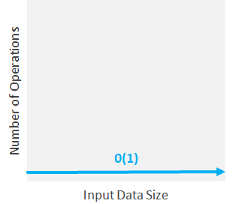
Constant Time Complexity: O(1)
When the complexity of time is constant (denoted as “O(1)”), the size of the input (n) is irrelevant. Algorithms with Constant Time Complexity run in a constant amount of time, regardless of its size n. They do not change their run-time in response to input data, making them the fastest algorithms available. These algorithms should not contain loops, recursions, or any other non-constant time function calls if they are to remain constant. The magnitude scale of run-time does not change for constant time algorithms: it is always 1.
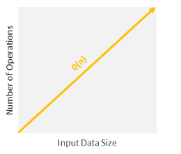
Linear Time Complexity: O(n)
When the running time of an algorithm increases linearly with regard to the length of input, it is said to have linear time complexity. When a function checks all of the values in an input data set, such a function has with this order, the time complexity is O(n).
A procedure that adds up all the elements of a list, for example, requires time proportional to the length of the list if the adding time is constant or, at the very least, bounded by a constant.
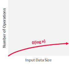
Logarithmic Time Complexity: O(log n)
When an algorithm reduces the impact of each input data set step, it is said to have a logarithmic time scale complexity. This indicates that the number of operations is not equal to the input size. As the dimension of the input increases, the number of operations decreases. Binary trees and binary search functions contain algorithms with logarithmic time complexity. This involves searching for a given value by separating in an array it in two and starting the search in one of the splits. This makes sure that the process is not performed with every data element.
Dictionary search provides an example of logarithmic time. Consider a dictionary D that has n entries in alphabetical order. We assume that for 1 ≤ k ≤ n, one can access the kth entry of the dictionary in a set amount of time. Let D(k) represent the k-th entry. According to these hypotheses, the test to see if a word w is in the dictionary could be performed in logarithmic time.
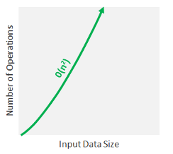
Quadratic Time Complexity: O(n²)
A non-linear time complexity algorithm is one whose The length of the input increases non-linearly (n2) with the length of the running time. In general, nested loops fall under the O(n) time complexity order, where one loop takes O(n) , and if the function includes a loop within a loop, it falls under the O(n)*O(n) = O(n2) time complexity order.
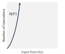
Exponential Time Complexity: O(2n)
Exponential (base 2) running time means that an algorithm's calculations double every time the input increases. Examples of exponential time complexity are like power set: locating all of a set's subsets, Fibonacci sequence etc.
Sorting Algorithms
A sorting algorithm is a computer science algorithm that arranges the elements of a list in a specific order.
- Heap Sort
Heapsort is a much faster variant of selection sort. It also performs by determining the list's largest (or smallest) element ,putting it at the end (or beginning) of the list, and then proceeding with the rest of the list, but it does so more productively by using a heap, a type of binary tree. When switching a data list to a heap, the root node is indeed the largest (or smallest) element. When it is excluded and shifted to the end of the list, the heap is reorganized so that the largest remaining element becomes the root. Identifying the next largest element on the heap needs to take O(log n) time, rather than O(n) for a linear scan as in simple selection sort. Finding the next largest element on the heap takes O(log n) time, rather than O(n) for a linear scan as in simple selection sort.
- Bubble Sort
Bubble Sort is a simple algorithm for sorting an array of n elements with a given set of n elements. Bubble Sort relates each element individually and sorts them based on their values.
If the given array must be sorted in ascending order, bubble sort will begin by comparing the first and second elements of the array; if the first element is more than the second element, it will swap both elements, and then compare the second and third elements, and so on.
It is referred to as bubble sort because, with each complete iteration, the most significant element in the given array bubbles up to the final position or the highest index, similar to how a water bubble expands to the water's surface. If we have n elements in total,, we must repeat this process n-1 times.If we have a total of n elements, we must repeat this process n-1 times.
- Merge Sort
Merge Sort uses the divide and conquer rule is used to recursively sort a given set of numbers/elements, which saves time. Merge Sort segregates an unsorted array of n elements into n subarrays, each with one element, because a single element is always sorted in itself. Then it merges these subarrays to repetitively generate new sorted subarrays, until a single fully sorted array is produced.
- Quick Sort
Quicksort employs a divide-and-conquer strategy. It involves taking a 'pivot' element from the array and separating the remaining elements into two sub-arrays based on whether they are less than or greater than the pivot. As a result, it is also known as partition-exchange sort. Formal paraphrase after that, the sub-arrays are sorted in a recursive manner. This can be done in-place, requiring small additional amounts of memory to perform the sorting.
Space Complexity
The portion of memory required to solve a single instance of a computational problem as a function of input characteristics is defined as an algorithm's or a computer program's space complexity.
Worst-Case complexity
In computer science, the worst-case complexity (usually denoted in asymptotic notation) measures the resources (e.g., running time, memory) that an algorithm requires given an arbitrary size input (commonly denoted as n or N).It provides an upper limit on the algorithm's resource requirements.
Common Mistakes
- Time and space complexity depends on lots of things like hardware, operating system, processors, etc. However, we don't consider any of these factors while analyzing the algorithm. We will only consider the duration of execution of an algorithm.
- The algorithm receives an unlabeled example.
Context and Applications
This topic is significant in the professional exams for both undergraduate and graduate courses, especially for
- Bachelors in Technology (Computer Science)
- Masters in Technology (Computer Science)
- Bachelors in Science (Computer Science)
- Masters in Science (Computer Science)
Related Concepts
- Space complexity.
- Average-case complexity.
- Asymptotic behavior.
Want more help with your computer science homework?
*Response times may vary by subject and question complexity. Median response time is 34 minutes for paid subscribers and may be longer for promotional offers.
Search. Solve. Succeed!
Study smarter access to millions of step-by step textbook solutions, our Q&A library, and AI powered Math Solver. Plus, you get 30 questions to ask an expert each month.
Time Complexity Homework Questions from Fellow Students
Browse our recently answered Time Complexity homework questions.
Search. Solve. Succeed!
Study smarter access to millions of step-by step textbook solutions, our Q&A library, and AI powered Math Solver. Plus, you get 30 questions to ask an expert each month.