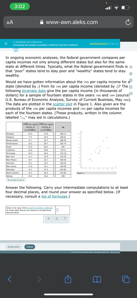
1980 per capita 1999 per capita income, x income, y xy (in $1000s) (in $1000s) ichigan Alabama 10.4 27.8 289.12 7.9 22.9 180.91 Rhode Island 9.7 29.7 288.09 Pennsylvania Texas California Minnesota 10.2 28.7 292.74 10.0 26.5 265 12.0 29.8 357.6 10.3 30.6 315.18 New York 11.1 33.9 376.29 New Mexico 8.4 22.1 185.64 8.2 23.2 Kentucky New Jersey 190.24 11.8 36.1 425.98 4. Nebraska 9.3 27.4 254.82 North Carolina 8.2 26.2 214.84 Figure 1 cansas 10.0 26.6 266 Send data to Excel

Big Ideas Math A Bridge To Success Algebra 1: Student Edition 2015
1st Edition
ISBN:9781680331141
Author:HOUGHTON MIFFLIN HARCOURT
Publisher:HOUGHTON MIFFLIN HARCOURT
Chapter4: Writing Linear Equations
Section4.5: Analyzing Lines Of Fit
Problem 25E
icon
Related questions
icon
Concept explainers
Topic Video
Question
100%
3:02
AA
www-awn.aleks.com
O REGRESSION AND CORRELATION
Computing the sample correlation coefficient and the coefficien.
In ongoing economic analyses, the federal government compares per
capita incomes not only among different states but also for the same
state at different times. Typically, what the federal government finds is
that "poor" states tend to stay poor and "wealthy" states tend to stay
wealthy.
Would we have gotten information about the 1999 per capita income for a
state (denoted by y) from its 1980 per capita income (denoted by x)? The O
following bivariate data give the per capita income (in thousands of
dollars) for a sample of fourteen states in the years 1980 and 1999 (source!
U.S. Bureau of Economic Analysis, Survey of Current Business, May 2000).
The data are plotted in the scatter plot in Figure 1. Also given are the
products of the 1980 per capita incomes and 1999 per capita incomes for
each of the fourteen states. (These products, written in the column
labelled "xy," may aid in calculations.)
1980 per capita 1999 per capita
income, x
income, y
ху
(in S1000s)
(in $1000s)
Michigan
Alabama
10.4
27.8
289.12
38-
7.9
22.9
180.91
Rhode Island
9.7
29.7
288.09
34-
Pennsylvania
10.2
28.7
292.74
32
Texas
10.0
26.5
265
30.
ICalifornia
12.0
29.8
357.6
25.
Minnesota
10.3
30.6
315.18
26
New York
New Mexico
11.1
33.9
376.29
24
8.4
22.1
185.64
22
Kentucky
8.2
23.2
190.24
20
New Jersey
11.8
36.1
425.98
Nebraska
9.3
27.4
254.82
North Carolina
8.2
26.2
214.84
Figure 1
Kansas
10.0
26.6
266
Send data to Excel
Answer the following. Carry your intermediate computations to at least
four decimal places, and round your answer as specified below. (If
necessary, consult a list of formulas.)
What is the value of the sample.correlation.coefficient
for these data? Round your answer to at least three
decimal places.
Explanation
Check
O 2021 McGraw-Hil Education. A Rights Reserved. Terms of Use
Transcribed Image Text:3:02 AA www-awn.aleks.com O REGRESSION AND CORRELATION Computing the sample correlation coefficient and the coefficien. In ongoing economic analyses, the federal government compares per capita incomes not only among different states but also for the same state at different times. Typically, what the federal government finds is that "poor" states tend to stay poor and "wealthy" states tend to stay wealthy. Would we have gotten information about the 1999 per capita income for a state (denoted by y) from its 1980 per capita income (denoted by x)? The O following bivariate data give the per capita income (in thousands of dollars) for a sample of fourteen states in the years 1980 and 1999 (source! U.S. Bureau of Economic Analysis, Survey of Current Business, May 2000). The data are plotted in the scatter plot in Figure 1. Also given are the products of the 1980 per capita incomes and 1999 per capita incomes for each of the fourteen states. (These products, written in the column labelled "xy," may aid in calculations.) 1980 per capita 1999 per capita income, x income, y ху (in S1000s) (in $1000s) Michigan Alabama 10.4 27.8 289.12 38- 7.9 22.9 180.91 Rhode Island 9.7 29.7 288.09 34- Pennsylvania 10.2 28.7 292.74 32 Texas 10.0 26.5 265 30. ICalifornia 12.0 29.8 357.6 25. Minnesota 10.3 30.6 315.18 26 New York New Mexico 11.1 33.9 376.29 24 8.4 22.1 185.64 22 Kentucky 8.2 23.2 190.24 20 New Jersey 11.8 36.1 425.98 Nebraska 9.3 27.4 254.82 North Carolina 8.2 26.2 214.84 Figure 1 Kansas 10.0 26.6 266 Send data to Excel Answer the following. Carry your intermediate computations to at least four decimal places, and round your answer as specified below. (If necessary, consult a list of formulas.) What is the value of the sample.correlation.coefficient for these data? Round your answer to at least three decimal places. Explanation Check O 2021 McGraw-Hil Education. A Rights Reserved. Terms of Use
Expert Solution
trending now

Trending now

This is a popular solution!

steps

Step by step

Solved in 2 steps

Blurred answer
Knowledge Booster
Application of Algebra
Learn more about
Need a deep-dive on the concept behind this application? Look no further. Learn more about this topic, statistics and related others by exploring similar questions and additional content below.
Similar questions
Recommended textbooks for you
Big Ideas Math A Bridge To Success Algebra 1: Stu…
Algebra
ISBN:
9781680331141
Author:
HOUGHTON MIFFLIN HARCOURT
Publisher:
Houghton Mifflin Harcourt