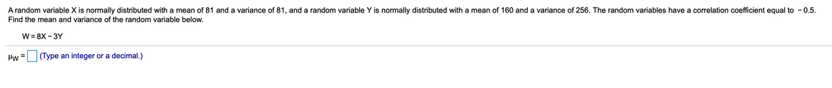
A random variable X is normally distributed with a mean of 81 and a variance of 81, and a random variable Y is normally distributed with a mean of 160 and a variance of 256. The random variables have a correlation coefficient equal to - 0.5. Find the mean and variance of the random variable below. W= 8X - 3Y Pw= (Type an integer or a decimal.)

Please write clearly.   Thank you.

The systolic blood pressure of individuals is thought to be related to both age and weight. Let the systolic blood pressure, age, and weight be represented by the variables x1, x2, and x3, respectively. Suppose that Minitab was used to generate the following descriptive statistics, correlations, and regression analysis for a random sample of 15 individuals.  Descriptive Statistics Variable N Mean Median TrMean StDev SE Mean x1 15 158.42 158.72 158.42 3.127 0.807388 x2 15 65.95 66.45 65.95 1.091 0.281695 x3 15 187.23 186.63 187.23 4.171 1.076948   Variable Minimum Maximum Q1 Q3 x1 124 174 135.828 166.400 x2 41 80 47.088 77.579 x3 124 244 142.885 223.525   Correlations (Pearson)   x1 x2 x2 0.829   x3 0.860 0.661 Regression Analysis  The regression equation is  x1 = 0.837 + 1.120x2 + 0.928x3    Predictor Coef StDev T P…

estion 3 of 38 university and gathers their freshman year GPA data and the high school SAI score reported on each of their college applications. He produces a scatterplot with SAT scores on the horizontal axis and GPA on the vertical axis. The data has a linear correlation coefficient of 0.506701. Additional sample statistics are summarized in the table below. Variable Sample Sample standard Variable description mean deviation high school SAT score x 1504.291401 Sx = 105.782904 %3D y freshman year GPA y = 3.240805 Sy = 0.441205 r = 0.506701 slope 0.002113 Determine the y-intercept, a, of the least-squares regression line for this data. Give your answer precise to at least four decimal places. tems of use Thelp about us குசங் careers 2:30 PM 10/24/20 o耳 国 @ hp

A history instructor has given the same pretest and the same final examination each semester. he is interested in determining if there is a relationship between the scores of the two tests. he computes the linear correlation coefficient and notes that it is 1.15. what does the correlation coefficient value tells the instructor? a. there is a strong positive correlation between the test b. there is a strong negative correlation between the test c. the history instructor has made a computational error d. the correlation is something other than linear

The maximum weights (in kilograms) for which one repetition of a half-squat can be performed and the jump heights (in centimeters) for 12 international soccer players are given in the accompanying table. The correlation coefficient, rounded to three decimal places, is r=0.692. At a =0.05, is there enough evidence to conclude that there is a significant linear correlation between the variables? E Click the icon to view the soccer player data. Determine the null and alternative hypotheses. Ho: p o Maximum Weights and Jump Heights Ha: p o Maximum Jump height, y Determine the critical value(s). weight, x 190 60 to = (Round to three decimal places as needed. Use a comma to separate answers as needed.) 185 56 155 55 Determine the standardized test statistic. 180 59 175 55 t= (Round to three decimal places as needed.) 170 65 What is the conclusion? 150 52 160 52 Ho. There V enough evidence at the 5% level of significance to conclude that there is a significant linear correlation between the…

Which of the following values represents the weakest correlation between two variables? о г= -0.17 г= 0.07 K r=0.45 r=-0.62 r = 0.81 00000

We give the total variation, the unexplained variation (SSE), and the least squares point estimate b1 .    Total variation = 13.459; SSE = 2.806; b1 = 2.6652       Click here for the Excel Data File   Using the information given, find the explained variation, the simple coefficient of determination (r2), and the simple correlation coefficient (r). Interpret r2. (Round your answers to 3 decimal places. Round your percent to 1 decimal place.)          Explained variation      r2      r            % of the variation in demand can be explained by variation in price differential.

Suppose Y1, Y2 and 3Y are not correlated variables, however, have the same standard deviation. Show that correlation between Y1 +  Y2 and  Y2 +  Y3 is equal to half. Whether correlation coefficient is zero or not

A researcher computes the correlation coefficient r= 0.4212 for an explanatory and response variable. What proportion of the changes in the response variables value is accounted for by the change in the explanatory variable's value? Give your answer to four decimal places.