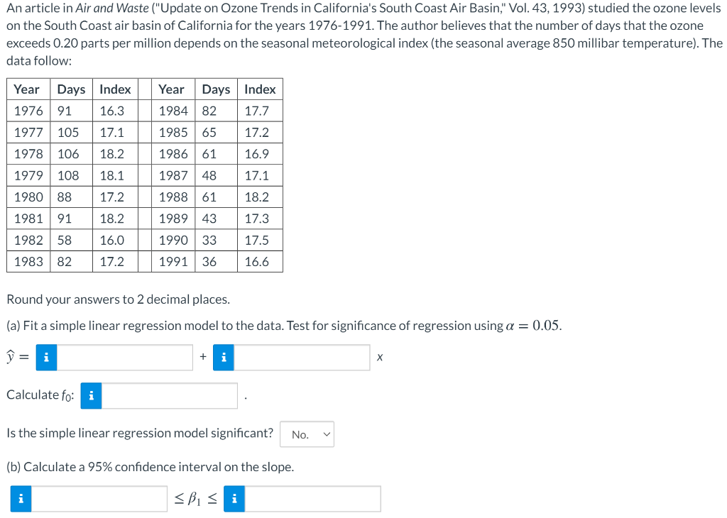
An article in Air and Waste ("Update on Ozone Trends in California's South Coast Air Basin," Vol. 43, 1993) studied the ozone levels on the South Coast air basin of California for the years 1976-1991. The author believes that the number of days that the ozone exceeds 0.20 parts per million depends on the seasonal meteorological index (the seasonal average 850 millibar temperature). The data follow: Year Days Index 1976 91 16.3 17.1 1977 105 1978 106 18.2 1979 108 18.1 1980 88 17.2 1981 91 18.2 1982 58 16.0 1983 82 17.2 Year Days Index 1984 82 17.7 1985 65 17.2 1986 61 16.9 1987 48 17.1 1988 61 18.2 1989 43 17.3 1990 33 17.5 1991 36 16.6 Round your answers to 2 decimal places. (a) Fit a simple linear regression model to the data. Test for significance of regression using a = 0.05. y = i Calculate fo: i + i Is the simple linear regression model significant? No. (b) Calculate a 95% confidence interval on the slope. ≤B₁ ≤i X

(1)Data was collected for 300 fish from the North Atlantic. The length of the fish (in mm) is summarized in the GFDT below.  Lenght (mm) Frequency 80 - 99 1 100 - 119 16 120 - 139 71 140 - 159 108 160 - 179 83 180 - 199 18 200 - 219 3 What is the upper class limit for the seventh class?upper class limit =

Consider the following data: Year Answer Deaths Number of Deaths in the U.S. by Drug Overdose 2000 2001 2002 2003 2004 2005 2006 2007 2008 17,035 17,510 14,316 13,382 17,756 14,516 11,155 18,656 16,643 Step 1 of 2: Find the two-period moving average for the year 2008. If necessary, round your answer to one decimal place.

The following frequency table summarizes a set of data. What is the five-number summary? Value   Frequency  7 1 8 1 9 3 10 1 13 3 15 3 16 2 17 1

An article reported on a​ long-term study of the effects of hurricanes on tropical streams of a forest. The study shows that a hurricane had a significant impact on stream water chemistry. The following shows a sample of 10 ammonia fluxes in the first year after the hurricane. Data are in kilograms per hectare per year. Complete parts​ (a) through​ (c) below.   98 80 145 145 174 115 58 58 87 158       find mean median and mode if no mode put no

The following table lists average high temperatures (° F) in January and in July for selected cities in the United States: Jan. hi. 45.9 July hi. 89.5 City July hi. City Nashville Jan. hi Atlanta 50.4 88 Baltimore 40.2 87.2 New Orleans 60.8 90.6 Boston 35.7 81.8 New York 37.6 85.2 Chicago 29 83.7 Philadelphia 37.9 82.6 Cleveland 31.9 82.4 Phoenix 65.9 105.9 Dallas 54.1 96.5 33.7 82.6 Pittsburgh St. Louis Salt Lake City San Diego Denver 43.2 88.2 37.7 89.3 Detroit 30.3 83.3 36.4 92.2 Houston 61 92.7 65.9 76.2 Kansas City Los Angeles 34.7 88.7 San Francisco 55.6 71.6 65.7 75.3 Seattle 45 75.2 Miami 75.2 89 Washington 42.3 88.5 Minneapolis 20.7 84 Which dataset exhibits more dispersion: the Jan. hi data or the July hi data? Explain your reasoning.

Consider the following data representing the price of refrigerators (in dollars). 1260, 1446, 1106, 1269, 1443, 1424, 1118, 1132, 1177, 1115, 1156, 1262, 1215, 1236, 1243, 1169, 1437, 1191, 1401, 1439, 1365 Answer Class 1093-1152 1153-1212 1213-1272 1273-1332 1333-1392 1393-1452 Price of Refrigerators (in Dollars) Frequency Relative Frequency Cumulative Frequency Step 3 of 4: Calculate the relative frequency of the sixth class. Determine your answer as a simplified fraction. Tables Keybe Previous

Consider the following data representing the price of refrigerators (in dollars). 1260, 1446, 1106, 1269, 1443, 1424, 1118, 1132, 1177, 1115, 1156, 1262, 1215, 1236, 1243, 1169, 1437, 1191, 1401, 1439, 1365 Answer Class 1093-1152 1153-1212 1213-1272 1273-1332 1333-1392 1393-1452 Step 2 of 4: Determine the frequency of the first class. Price of Refrigerators (in Dollars) Frequency Relative Frequency Cumulative Frequency Tables

An investigation of the properties of bricks used to line aluminum smelter pots was published in an article. Six different commercial bricks were evaluated. The life span of a smelter pot depends on the porosity of the brick lining (the less porosity, the longer the life span); consequently, the researchers measured the apparent porosity of each brick specimen, as well as the mean pore diameter of each brick. See the table. Apparent Porosity (y). Mean Pore Diameter (x). Click the icon to view the table. Data table Mean Pore Diameter Apparent Porosity (%) (micrometers) Brick Interpret the y-intercept of the line. Choose the correct answer below. 18.7 12.0 В 18.3 9.8 O A. The y-intercept is Bo- This value has no meaning because 0 is not in the observed range of the independent variable mean pore diameter. 16.3 7.3 6.9 5.4 O B. The y-intercept is Bo: For each unit increase in mean pore diameter, the mean porosity is estimated to increase by B0- 17.2 10.9 O C. There is not enough…

Data was collected for 300 fish from the North Atlantic. The length of the fish (in mm) is summarized in the GFDT below.   Lengths (mm)      Frequency    180 - 184 1 185 - 189 16 190 - 194 71 195 - 199 108 200 - 204 83 205 - 209 18 210 - 214 3 What is the lower class limit for the sixth class?lower class limit =