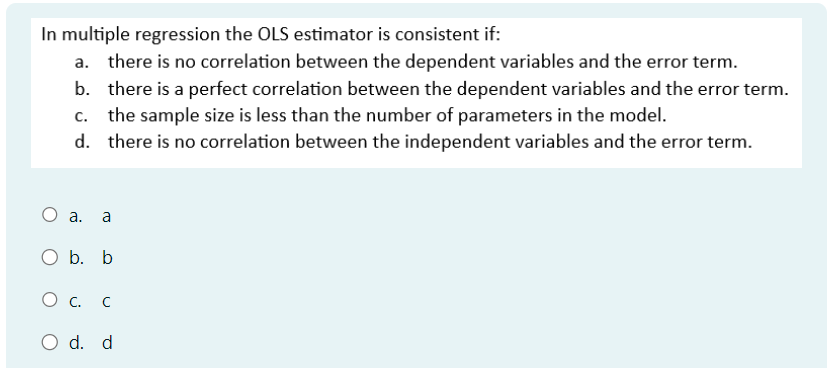
In multiple regression the OLS estimator is consistent if: there is no correlation between the dependent variables and the error term. b. there is a perfect correlation between the dependent variables and the error term. c. the sample size is less than the number of parameters in the model. d. there is no correlation between the independent variables and the error term. O a. a O b. b О с. C ○ d. d

wages = B1 + B2educ + ßzexper + e where wages denotes hourly wages. We estimate the regression in R and obtain the output ## Coefficients: ## Estimate Std. Error t value Pr(>|t|) ## (Intercept) 2.0 1.0 2 0.0455 * ## educ 0.5 0.5 1 0.3173 ## exper 2.0 0.5 4 6.33e-05 *** ## --- ## Signif. codes: ****' 0. 001 '**' 0.01 **' 0.05 ' 0.1 ' ' 1 Build a 90% confidence interval for B3 using a normal approximation. (Use that if Z ~ N(0, 1) and z1-a satisfies P(Z > z1-a) = a, then zo9 = 1.28, zo95 = 1.64, Z0.975 = 1.96, zo.99 = 2.33, and z0.995 = 2.58). Oa. [2 – 1.64 x (0.5), 2 + 1.64 x (0.5)] O b. [2 – 1.28 × (0.5), 2 + 1.28 x (0.5)] c. [2 – 1.28 x (0.5)², 2 + 1.28 × (0.5)²] O d. [2 – 1.64 × (0.5)², 2 + 1.64 × (0.5)²] O e. [2 – 1.96 × (0.5)², 2 + 1.96 × (0.5)²] O f. [2 – 1.96 × (0.5), 2 + 1.96 × (0.5)]

In a regression model, if the variance of the dependent variable, y, conditional on an explanatory variable, x, or Var(y/x), is not constant, a. the t statistics are invalid and the confidence intervals are valid for small sample sizes. b. the t statistics are valid and the confidence intervals are invalid for small sample sizes. c. the t statistics and the confidence intervals are valid no matter how large the sample size. d. the t statistics and the confidence intervals are both invalid no matter how large the sample size. O a. a O b. b О с. C ○ d. d

Determine the PRF.

You are interested in how the number of hours a high school student has to work in an outside job has on their GPA. In your regression you want to control for high school standing and so you run the following regression: GPA = 3.4 0.03 * HrsWrk - 0.7 * Frosh - 0.3 * Soph +0.1 * Junior (1.1) (0.013) (0.23) (0.14) (0.08) where HrsWrk is the number of hours the student works per week, and Frosh, Soph, and Junior are dummy variables for the student's class standing. a) If you include a dummy variable for seniors, that would cause a Hint: type one word in each blank. For the rest of questions, type a number in one decimal place. b) The expected GPA of a Sophomore who works 10 hours per week is c) The expected GPA of a Senior who works 10 hours per week is d) If Dom and Sarah work the same number of hours per week, but Dom is a Junior and Sarah is a Freshman. Dom is expected to have a higher GPA than Sarah. e) Suppose you rewrite the regression as: problem. GPA = ₁HrsWrk + ß2Frosh + B2Soph +…

In an OLS regression, which value represents the "best" R2 in terms of explained variance in the dependent variable?  A. 2.53 B. 16.22 C. .001 D. 0.53

Help!

You estimated a regression with the following output.         Source |       SS           df       MS      Number of obs   =       411 -------------+----------------------------------   F(1, 409)       =   4098.54        Model |  22574040.7         1  22574040.7   Prob > F        =    0.0000     Residual |  2252702.97       409  5507.83122   R-squared       =    0.9093 -------------+----------------------------------   Adj R-squared   =    0.9090        Total |  24826743.7       410  60553.0334   Root MSE        =    74.215   ------------------------------------------------------------------------------            Y |      Coef.   Std. Err.      t    P>|t|     [95% Conf. Interval] -------------+----------------------------------------------------------------            X |   6.727341   .1050822    64.02   0.000     6.520772    6.933909        _cons |  -.7552724    9.26027    -0.08   0.935    -18.95894    17.44839…

QUESTION 10 Answer questions 10 to 16 based on the regression outputs given in Table 1& 2. Table 1 DATA4-1: Data on single family homes in University City community of San Diego, in 1990. price - sale price in thousands of dollars (Range 199. 9 505) sqft - square feet of living area (Range 1065 - 3000) Table 2 Model 1: OLS, using observations 1-14 Dependent variable: price coefficient std. error t-ratio p-value 52. 3509 0.138750 37. 2855 0.0187329 0. 1857 8. 20e-06 *** const sqft 7. 407 Me dependent var Sun squared resid R-squared F(1, 12) Log-likelihood Schwarz criterion 317. 4929 18273. 57 0. 820522 54. 86051 -70. 08421 145. 4465 Hannan-Quinn S.D. dependent var S.E. of regression Adjusted R-squared P-value (F) Akaike criterion 88. 49816 39. 02304 0. 805565 8. 20e-06 144. 1684 144. 0501 There are observations included in this dataset. It is a. data. O 12; cross-sectional 13; time-series data 14; cross-sectional In this regression model, sale price of a single-family house is the. the…

The data for this question is given in the file 1.Q1.xlsx(see image)  and it refers to data for some cities X1 = total overall reported crime rate per 1 million residents X3 = annual police funding in $/resident X7 = % of people 25 years+ with at least 4 years of college   (a) Estimate a regression with X1 as the dependent variable and X3 and X7 as the independent variables. (b) Will additional education help to reduce total overall crime (lead to a statistically significant reduction in crime)? Please explain. (c) Will an increase in funding for the police departments help reduce total overall crime (lead to a statistically significant reduction in total overall crime)? Please explain. (d) If you were asked to recommend a policy to reduce crime, then, based only on the above regression results, would you choose to invest in education (local schools) or in additional funding for the police? Please explain.