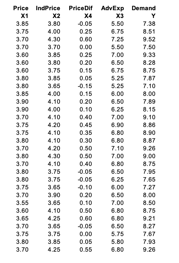
PriceIndPrice PriceDifAdvExp DemandX1X2X4X3Y3.853.80-0.055.507.383.754.000.256.758.513.704.300.607.259.523.703.700.005.507.503.603.850.257.009.333.603.800.206.508.283.603.750.156.758.753.803.850.055.257.873.803.65-0.155.257.103.854.000.156.008.003.904.100.206.507.893.904.000.106.258.153.704.100.407.009.103.754.200.456.908.863.754.100.356.808.903.804.100.306.808.873.704.200.507.109.263.804.300.507.009.003.704.100.406.808.753.803.75-0.056.507.953.803.75-0.056.257.653.753.65-0.106.007.273.703.900.206.508.003.553.650.107.008.503.604.100.506.808.753.654.250.606.809.213.703.65-0.056.508.273.753.750.005.757.673.803.850.055.807.933.704.250.556.809.26 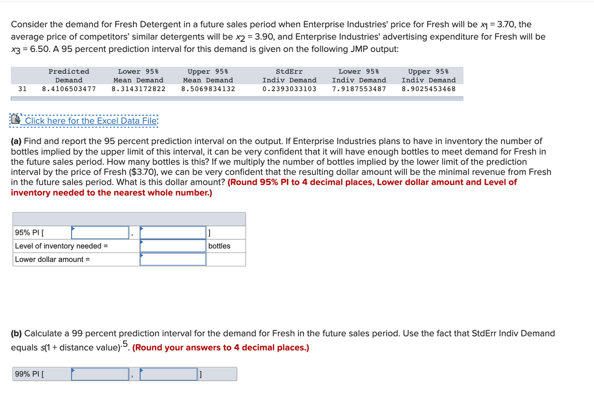Consider the demand for Fresh Detergent in a future sales period when Enterprise Industries' price for Fresh will be x1 = 3.70, theaverage price of competitors' similar detergents will be x2 = 3.90, and Enterprise Industries' advertising expenditure for Fresh will bex3 = 6.50. A 95 percent prediction interval for this demand is given on the following JMP output:%3DPredictedLower 95%Upper 95%Mean DemandUpper 95%Indiv DemandStdErrLower 95%DemandMean DemandIndiv DemandIndiv Demand318.41065034778.31431728228.50698341320.23930331037.91875534878.9025453468E Click here for the Excel Data File;(a) Find and report the 95 percent prediction interval on the output. If Enterprise Industries plans to have in inventory the number ofbottles implied by the upper limit of this interval, it can be very confident that it will have enough bottles to meet demand for Fresh inthe future sales period. How many bottles is this? If we multiply the number of bottles implied by the lower limit of the predictioninterval by the price of Fresh ($3.70), we can be very confident that the resulting dollar amount will be the minimal revenue from Freshin the future sales period. What is this dollar amount? (Round 95% PI to 4 decimal places, Lower dollar amount and Level ofinventory needed to the nearest whole number.)95% PI [Level of inventory needed =bottlesLower dollar amount =(b) Calculate a 99 percent prediction interval for the demand for Fresh in the future sales period. Use the fact that StdErr Indiv Demandequals s(1 + distance value)5. (Round your answers to 4 decimal places.)99% PI [

Since you have asked multiple questions, we will solve the first question for you. If you want any…

Answered: Price IndPrice PriceDif AdvExp Demand…

MATLAB: An Introduction with Applications

6th Edition

ISBN:9781119256830

Author:Amos Gilat

Publisher:Amos Gilat

Chapter1: Starting With Matlab

Section: Chapter Questions

Problem 1P

See similar textbooks

Similar questions

Compute the forecasted values for Yt for July and August in 2020 by using the modelsstated in (c) and (d)
Floyd Distributors, Inc., provides a variety of auto parts to small local garages. Floyd purchases parts from manufacturers according to the EOQ model and then ships the parts from a regional warehouse direct to its customers. For a particular type of muffler, Floyd's EOQ analysis recommends orders with Q* = 20 to satisfy an annual demand of 180 mufflers. Floyd's has 250 working days per year, and the lead time averages 15 days.Note: Use Appendix B to identify the areas for the standard normal distribution. What is the reorder point if Floyd assumes a constant demand rate? If required, round your answer up to the nearest whole number. r = fill in the blank 1 Suppose that an analysis of Floyd's muffler demand shows that the lead-time demand follows a normal probability distribution with µ = 12 and σ = 2.2. If Floyd's management can tolerate one stock-out per year, what is the revised reorder point? If required, round your answer up to the nearest whole number. r = fill in the blank…
Based on the EViews results above, answer the following questions.a. What is your comments on the diagnostic tests of the model? i. Autocorrelation test ii. Heteroscedasticity test iii. Normality
Assume that as a portfolio manager the beta of your portfolio is 1.15 and that your performance is exactly on target with the SML data under condition 1. If the true SML data is given by condition 2, how much does your performance differ from the true SML? (1) RFR = 0.0625 Rm(proxy) = 0.12 (2) RK = 0.078 Rm(true) = 0.10
The following data show the results of random sample of 10 batches of one pattern of product: Sample Batch Size X Support Costs Y 1 10 10$ 2 12 15 3 15 20 4 20 22 5 10 15 6 25 25 7 20 30 8 12 10 9 15 20 10 30 30 Calculate: Using High and Low method and predict Variable cost and fixed cost of the above information.
The manager of the purchasing department of a large banking organization would like to develop a model to predict the amount of time it takes to process invoices. Data are collected from a sample of 30 days with the following results: Relating time to invoices processed. Day Invoices Processed Completion Time (hours) Day Invoices Processed Completion Time (hours) 1 149 2.1 16 169 2.5 2 60 1.8 17 190 2.9 3 188 2.3 18 233 3.4 4 19 0.3 19 289 4.1 5 201 2.7 20 45 1.2 6 58 1.0 21 193 2.5 7 77 1.7 22 70 1.8 8 222…
Find the critical value, the computed t-value, and whether to reject or accept the null hypothesis.
A study was conducted to demonstrate that soybeans inoculated with nitrogen-fixing bacteria yield more and grow adequately without expensive environmentally deleterious synthesized fertilizers. The trial was conducted under controlled conditions with uniform amounts of soil. The initial hypothesis was that inoculated plants would outperform their uninoculated counterparts. This assumption is based on the facts that plants need nitrogen to manufacture vital proteins and amino acids and that nitrogen-fixing bacteria would make more of this substance available to plants, increasing their size and yield. There were 8 inoculated plants (I) and 8 uninoculated plants (U). The plant yield as measured by pod weight for each plant is given in Table 2.20 Here are the questions I would like explanations for. Please use STATA to compute answers!!!: 2.35. The objective is to compute appropriate descriptive statistics for I and Data set available U plants. 2.36. Use graphic methods to compare the…
A study was conducted to demonstrate that soybeans inoculated with nitrogen-fixing bacteria yield more and grow adequately without expensive environmentally deleterious synthesized fertilizers. The trial was conducted under controlled conditions with uniform amounts of soil. The initial hypothesis was that inoculated plants would outperform their uninoculated counterparts. This assumption is based on the facts that plants need nitrogen to manufacture vital proteins and amino acids and that nitrogen-fixing bacteria would make more of this substance available to plants, increasing their size and yield. There were 8 inoculated plants (I) and 8 uninoculated plants (U). The plant yield as measured by pod weight for each plant is given in Table 2.20. Compute appropriate descriptive statistics for I and Data set available U plants.
An urban community wants to show that the incidence of breast cancer is higher in their locality than in a neighboring rural area. (PCB levels were found to be higher in the soil of the urban community). If you find that in the urban community 20 out of 200 adult women have breast cancer and that in the rural community 10 out of 150 adult women have it, could you conclude, at a significance level of 0.05, that breast cancer is more prevalent in the urban community?1. The parameter of interest is:2. The hypotheses for this test are:3. The calculated test statistic is:4. The critical region is:5. Draw the critical region (make decision):6. It can be concluded that:
A study was conducted to assess the impact of nutrient enrichment on zooplankton densities in A & B Islands. An ecologist sampled populations of zooplankton in these two locations and observed the nutrient enrichment level was higher in A island when compared with the level in B island. It is predicted the zooplankton densities in A island will be greater than those found in B island.
Consider a cohort study to compare the mortality rate of myocardial infarction (MI) in men with sedentary work (exposed group) to men with physically active work (unexposed). If in the exposed, there were 36,000 person (man) years of observation and 126 deaths whereas the unexposed had 24,000 man-years of observation and 44 deaths. Compute the following a) Mortality rate in each cohort? b) What is the relative risk of dying, comparing these 2 groups? c) What is the attributable risk of sedentary work? d) What is the attributable benefit of physical activity? e) If we assume that MI is associated with the mortality in this cohort (causality), what proportion of the disease in the higher group is potentially preventable?

SEE MORE QUESTIONS

Recommended textbooks for you

MATLAB: An Introduction with Applications

Statistics

ISBN:

9781119256830

Author:

Amos Gilat

Publisher:

John Wiley & Sons Inc

Probability and Statistics for Engineering and th…

Statistics

ISBN:

9781305251809

Author:

Jay L. Devore

Publisher:

Cengage Learning

Statistics for The Behavioral Sciences (MindTap C…

Statistics

ISBN:

9781305504912

Author:

Frederick J Gravetter, Larry B. Wallnau

Publisher:

Cengage Learning

MATLAB: An Introduction with Applications

Statistics

ISBN:

9781119256830

Author:

Amos Gilat

Publisher:

John Wiley & Sons Inc

Probability and Statistics for Engineering and th…

Statistics

ISBN:

9781305251809

Author:

Jay L. Devore

Publisher:

Cengage Learning

Statistics for The Behavioral Sciences (MindTap C…

Statistics

ISBN:

9781305504912

Author:

Frederick J Gravetter, Larry B. Wallnau

Publisher:

Cengage Learning

Elementary Statistics: Picturing the World (7th E…

Statistics

ISBN:

9780134683416

Author:

Ron Larson, Betsy Farber

Publisher:

PEARSON

The Basic Practice of Statistics

Statistics

ISBN:

9781319042578

Author:

David S. Moore, William I. Notz, Michael A. Fligner

Publisher:

W. H. Freeman

Introduction to the Practice of Statistics

Statistics

ISBN:

9781319013387

Author:

David S. Moore, George P. McCabe, Bruce A. Craig

Publisher:

W. H. Freeman

SEE MORE TEXTBOOKS