
MATLAB: An Introduction with Applications
6th Edition
ISBN: 9781119256830
Author: Amos Gilat
Publisher: John Wiley & Sons Inc
expand_more
expand_more
format_list_bulleted
Related questions
Question
The table below shows a sample of waiting times (in days) for a heart transplant for two age groups. At α=0.05, can you conclude that the variances of the waiting times differ between the two age groups?
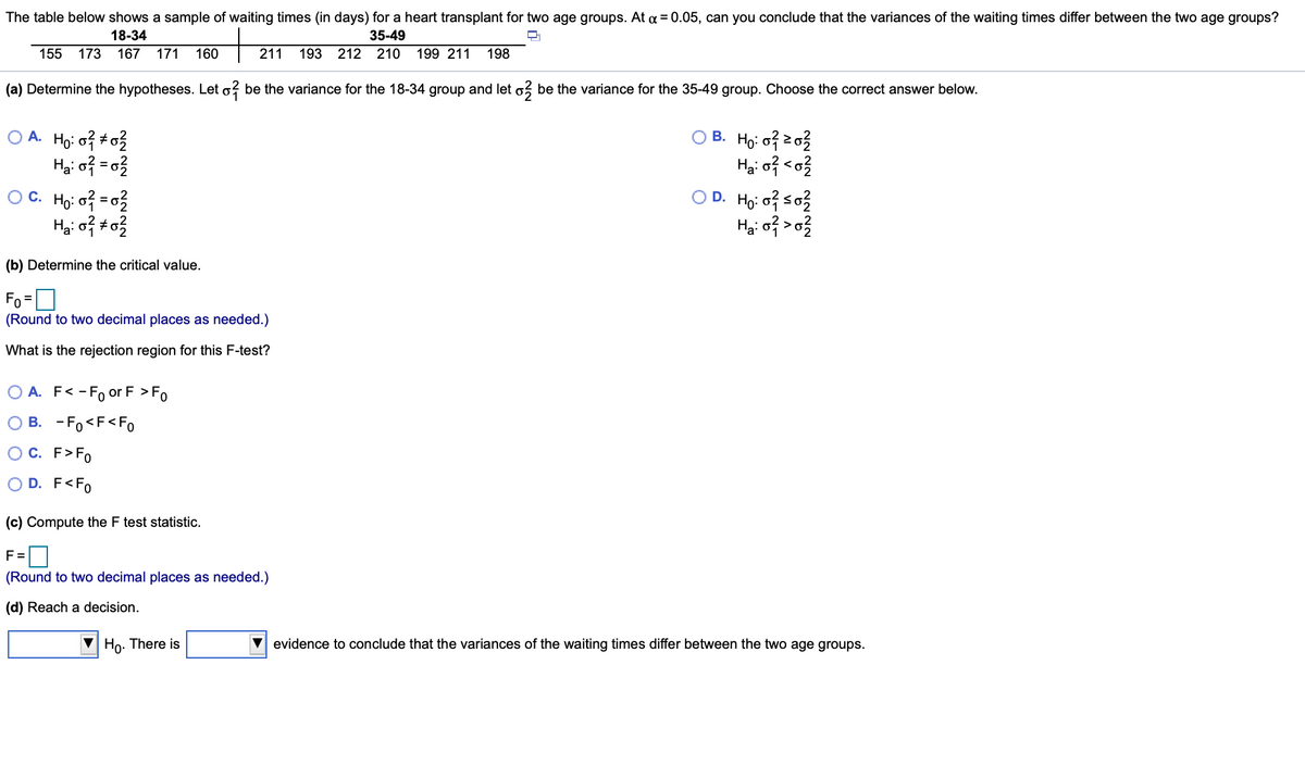

Transcribed Image Text:The table below shows a sample of waiting times (in days) for a heart transplant for two age groups. At a = 0.05, can you conclude that the variances of the waiting times differ between the two age groups?
18-34
35-49
155 173
167
171
160
211
193 212
210
199 211
198
(a) Determine the hypotheses. Let o? be the variance for the 18-34 group and let o? be the variance for the 35-49 group. Choose the correct answer below.
O A. Ho: of #o3
Hai of =o3
OC. Ho: o =02
B. Ho: of z03
Hại of <o}
O D. Ho: of so3
Hại of >o?
(b) Determine the critical value.
Fo =O
(Round to two decimal places as needed.)
%3D
What is the rejection region for this F-test?
O A. F< -Fo or F >Fo
О В. - Fo<F<Fo
OC. F>Fo
O D. F<Fo
(c) Compute the F test statistic.
F =
(Round to two decimal places as needed.)
(d) Reach a decision.
Ho. There is
evidence to conclude that the variances of the waiting times differ between the two age groups.
Expert Solution
This question has been solved!
Explore an expertly crafted, step-by-step solution for a thorough understanding of key concepts.

This is a popular solution

Trending nowThis is a popular solution!

Step by stepSolved in 4 steps

Knowledge Booster


Learn more about
Need a deep-dive on the concept behind this application? Look no further. Learn more about this topic, statistics and related others by exploring similar questions and additional content below.Similar questions
- A research study investigated the composition of wines from the Rhine and Moselle wine regionsof Germany. One component measured was the concentration of i-Butyl alcohol. The results ofthe study are listed in the following table:Region n i-Butyl alcohol (mg/100ml)Rhine 9 ̄x =5.32,s =2.24Moselle 14 ̄x =3.62,s =0.97(a) Assume that the underlying population variances from the two regions are identical. At the0.05 level of significance, test the null hypothesis that the mean concentration of i-Butylalcohol is the same for wines from the Rhine and Moselle regions.Construct a 95% confidence interval(b) Now assume that the underlying population variances from the two regions differ. At the 0.05level of significance, test the null hypothesis that the mean concentration of i-Butyl alcohol isthe same for wines from the Rhine and Moselle regions, construct a 95% confidence interval(c) If you were to provide a report to the investigators which of the above results would youinclude and why?arrow_forwardThe average age of the library books is μ = 20 in California. This distribution is negatively skewed. But the librarian at the local elementary school claims that, on average, the books in the library are more than 20 years old. To test this claim, this librarian takes a sample of n = 16 books and records the publication date for each. The sample produces an average age of M = 23.8 years with a variance of s² = 67.5. Do the data from this sample provide evidence that the age of books in this local elementary school is older than the average age of population? Use α = .01arrow_forwardThe Cadet is a popular model of sport utility vehicle, known for its relatively high resale value. The bivariate data given below were taken from a sample of Cadets, each bought new two years ago, and each sold used within the past month. For each Cadet in the sample, we have listed both the mileage x (in thousands of miles) that the Cadet had on its odometer at the time it was sold used and the price y (in thousands of dollars) at which the Cadet was sold used. With the aim of predicting the used selling price from the number of miles driven, we might examine the least-squares regression line, =y−41.990.51x . This line is shown in the scatter plot below. Based on the sample data and the regression line, complete the following. (a)For these data, mileages that are less than the mean of the mileages tend to be paired with used selling prices that are ▼(Choose one) the mean of the used selling prices. (b)According to the regression equation, for an increase of…arrow_forward
- Highway engineers in Ohio are painting white stripes on a highway. The stripes are supposed to be approximately 10 feet long. However, because of the machine, the operator, and the motion of the vehicle carrying the equipment, considerable variation occurs among the stripe lengths. Engineers claim that the variance of stripes should be less than 16 inches squared. At α = .05, use the sample lengths given here from 12 measured stripes (in feet and inches) to test the variance claim. Assume stripe length is normally distributed. (in feet) (in inches) 9.85 118.2 9.7 116.4 9.9 118.8 9.5 114 9.15 109.8 10.1 121.2 10 120 9.8 117.6 9.9 118.8 10.3 123.6 10.1 121.2 10.2 122.4 The appropriate test for this question is: a Z-test for the true variance of stripe length. a t-test for the true mean of stripe length. a Chi-square test…arrow_forwardA correlation of +.20 means that [blank] of the variance in the outcome variable is accounted for by the predictor variable.arrow_forwardThe average age at which adolescent girls reach their adult height is 16 years. Suppose you have a sample of 29 adolescent girls who are developmentally delayed, and who have an average age at which they reached their adult height of 17.8 years and a sample variance of 77.4 years. You want to test the hypothesis that adolescent girls who are developmentally delayed have a different age at which they reached their adult height than all adolescent girls. In order to calculate the t statistic, you first need to calculate the estimated standard error. The estimated standard error SM = (round to four decimals)arrow_forward
- The average age at which adolescent girls reach their adult height is 16 years. Suppose you have a sample of 29 adolescent girls who are developmentally delayed, and who have an average age at which they reached their adult height of 17.8 years and a sample variance of 77.4 years. You want to test the hypothesis that adolescent girls who are developmentally delayed have a different age at which they reached their adult height than all adolescent girls. In order to calculate the t statistic, you first need to calculate the estimated standard error. The estimated standard error SM= (round to four decimals)arrow_forwardThe mean age of 31 slot mechanic player is 51.3 years, and the standard deviation is 6.8 years.the mean age of a different sample of 35 roulette player is 54.8 year and standard deviation is 3.2 years. Can it be concluded at alpha = 0.01 that the mean age of slot machine players is less than those players roulette? Assume the variance are equal Step 1= Step 2= Step 3= Step 4=arrow_forwardThe data from an independent-measures research study produce a sample mean difference of 4 points, and each sample has a variance of 10. If there are n = 20 scores in each sample, then what is the estimated standard error of the difference between means?arrow_forward
- Records from previous years for a casualty insurance company show that its clients average a combined total of 1.9 auto accidents per day, with a variance of 0.31. The actuaries of the company claim that the current variance, oʻ, of the number of accidents per day is not equal to 0.31. A random sample of 17 recent days had a mean of 2 accidents per day with a variance of 0.62. If we assume that the number of accidents per day is approximately normally distributed, is there sufficient evidence to conclude, at the 0.05 level of significance, that the actuaries are correct? Perform a two-tailed test. Then complete the parts below. Carry your intermediate computations to three or more decimal places and round your answers as specified below. (If necessary, consult a list of formulas.) (a) State the null hypothesis H, and the alternative hypothesis H,. p H, :0 H, :0 (b) Determine the type of test statistic to use. (Choose one) ▼ D=0 OSO O20 (c) Find the value of the test statistic. (Round…arrow_forwardThe variability in the amounts of impurities present in a batch of chemical used for a particular process depends on the length of time the process is in operation. A manufacturer using two production lines, 1 and 2, has made a slight adjustment to line 2, hoping to reduce the variability as well as the average amount of impurities in the chemical. Samples of 25 and 25 measurements from the two batches yield 1.04, respectively 0.51 variances. Do the data present sufficient evidence to indicate that the process variability is less for line 2? Use 5% significance level. Conduct a hypothesis test of the airline executive’s belief. [α = 0.05]arrow_forwardA certain IQ test is known to have a population mean of 100 and standard deviation of 15 in the general population. You want to test whether psychology majors have a different average IQ than the population as a whole. Assume the variance of IQ is the same for Psych majors as it is in the general population. Suppose that Psychology majors actually have an average IQ of 108. If you do a 2-tailed test at α= .05 with a sample of 56 Psychology majors, you will be able to reject the null hypothesis if the mean IQ of your sample is below [L] or above [H]. Find L and H values. Options listed below. [L] answer choices: 96.08, 98.00, 103.92, 104.08, 110.00, 111.92. [H] Answer choices: 96.08, 98.00, 103.92, 104.08, 110.00, 111.92.arrow_forward
arrow_back_ios
SEE MORE QUESTIONS
arrow_forward_ios
Recommended textbooks for you
- MATLAB: An Introduction with ApplicationsStatisticsISBN:9781119256830Author:Amos GilatPublisher:John Wiley & Sons Inc
 Probability and Statistics for Engineering and th...StatisticsISBN:9781305251809Author:Jay L. DevorePublisher:Cengage Learning
 Statistics for The Behavioral Sciences (MindTap C...StatisticsISBN:9781305504912Author:Frederick J Gravetter, Larry B. WallnauPublisher:Cengage Learning
  Elementary Statistics: Picturing the World (7th E...StatisticsISBN:9780134683416Author:Ron Larson, Betsy FarberPublisher:PEARSON
 The Basic Practice of StatisticsStatisticsISBN:9781319042578Author:David S. Moore, William I. Notz, Michael A. FlignerPublisher:W. H. Freeman
 Introduction to the Practice of StatisticsStatisticsISBN:9781319013387Author:David S. Moore, George P. McCabe, Bruce A. CraigPublisher:W. H. Freeman
MATLAB: An Introduction with Applications
Statistics
ISBN:9781119256830
Author:Amos Gilat
Publisher:John Wiley & Sons Inc
Probability and Statistics for Engineering and th...
Statistics
ISBN:9781305251809
Author:Jay L. Devore
Publisher:Cengage Learning
Statistics for The Behavioral Sciences (MindTap C...
Statistics
ISBN:9781305504912
Author:Frederick J Gravetter, Larry B. Wallnau
Publisher:Cengage Learning
Elementary Statistics: Picturing the World (7th E...
Statistics
ISBN:9780134683416
Author:Ron Larson, Betsy Farber
Publisher:PEARSON
The Basic Practice of Statistics
Statistics
ISBN:9781319042578
Author:David S. Moore, William I. Notz, Michael A. Fligner
Publisher:W. H. Freeman
Introduction to the Practice of Statistics
Statistics
ISBN:9781319013387
Author:David S. Moore, George P. McCabe, Bruce A. Craig
Publisher:W. H. Freeman