Concept explainers
Videos
The following data give the lengths of time to failure for n = 88 radio transmitter-receivers:
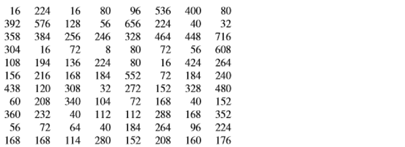
- a Use the
range to approximate s for the n = 88 lengths of time to failure. - b Construct a frequency histogram for the data. [Notice the tendency of the distribution to tail outward (skew) to the right.]
- c Use a calculator (or computer) to calculate
- d Calculate the intervals
empirical rule results. Note that the empirical rule provides a rather good description of these data, even though the distribution is highly skewed.
a.
Calculate the approximate value of s by using the range.
Answer to Problem 25SE
The approximate value of s by using the range is 177.
Explanation of Solution
An empirical rule suggests that the standard deviation is approximately one-fourth of the range.
The maximum observation is 716; the minimum observation is 8. Thus, the range is
Thus, the approximate value of s by using the range is
b.
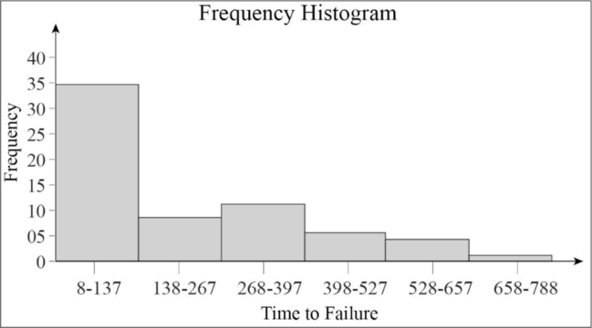
Make a frequency histogram for the given data.
Answer to Problem 25SE
The frequency histogram for the give data is obtained as follows:
Explanation of Solution
Calculation:
The lowest and highest values of the give data are 8 and 716, respectively.
Consider the class width for each interval is 130 units.
For convenience, start the class interval of the lowest class at 8 and end the class interval of the highest class at 788. Although the class intervals should ideally be continuous, for convenience, the classes have been taken as disjoint, such as 8 – 137, 138 – 267, etc. Note that, in the first class, both 8 and 137 are included, in the second class, both 138 and 267 are included, and so on.
Hence, the frequency distribution table of the class intervals for the given data.
| Time to Failure | Frequency |
| 8 – 137 | 35 |
| 138 – 267 | 28 |
| 268 – 397 | 13 |
| 398 – 527 | 6 |
| 528 – 657 | 5 |
| 658 – 788 | 1 |
| Total | 25 |
Graphical procedure:
Step-by-step procedure to draw the relative frequency histogram is given below:
- Draw the horizontal axis to represent the class intervals; mark the points listed under the column of “Time to Failure” in the above table.
- Draw the vertical axis to represent the frequencies; mark the points from 0 to 40, at intervals of 5, and label them.
- Corresponding to each class interval, draw a box with the height that is indicated under the column of “Frequency” in the above table.
- Under each box, label with the class interval that it represents.
The frequency histogram for the give data is obtained.
By carefully observing the histogram, it can be seen that there is a longer tail towards the higher values, which indicates a distribution that is skewed to the right.
c.
Calculate the values of
Answer to Problem 25SE
The value of
The value of s is 162.1728.
Explanation of Solution
The formula for the mean is,
Thus, the mean and standard deviation are obtained as follows:
| 16 | 256 |
| 392 | 153,664 |
| 358 | 128,164 |
| 304 | 92,416 |
| 108 | 11,664 |
| 156 | 24,336 |
| 438 | 191,844 |
| 60 | 3,600 |
| 360 | 129,600 |
| 56 | 3,136 |
| 168 | 28,224 |
| 224 | 50,176 |
| 576 | 331,776 |
| 384 | 147,456 |
| 16 | 256 |
| 194 | 37,636 |
| 216 | 46,656 |
| 120 | 14,400 |
| 208 | 43,264 |
| 232 | 53,824 |
| 72 | 5,184 |
| 168 | 28,224 |
| 16 | 256 |
| 128 | 16,384 |
| 256 | 65,536 |
| 72 | 5,184 |
| 136 | 18,496 |
| 168 | 28,224 |
| 308 | 94,864 |
| 340 | 115,600 |
| 40 | 1,600 |
| 64 | 4,096 |
| 114 | 12,996 |
| 80 | 6,400 |
| 56 | 3,136 |
| 246 | 60,516 |
| 8 | 64 |
| 224 | 50,176 |
| 184 | 33,856 |
| 32 | 1,024 |
| 104 | 10,816 |
| 112 | 12,544 |
| 40 | 1,600 |
| 280 | 78,400 |
| 96 | 9,216 |
| 656 | 430,336 |
| 328 | 107,584 |
| 80 | 6,400 |
| 80 | 6,400 |
| 552 | 304,704 |
| 272 | 73,984 |
| 72 | 5,184 |
| 112 | 12,544 |
| 184 | 33,856 |
| 152 | 23,104 |
| 536 | 287,296 |
| 224 | 50,176 |
| 464 | 215,296 |
| 72 | 5,184 |
| 16 | 256 |
| 72 | 5,184 |
| 152 | 23,104 |
| 168 | 28,224 |
| 288 | 82,944 |
| 264 | 69,696 |
| 208 | 43,264 |
| 400 | 160,000 |
| 40 | 1,600 |
| 448 | 200,704 |
| 56 | 3,136 |
| 424 | 179,776 |
| 184 | 33,856 |
| 328 | 107,584 |
| 40 | 1,600 |
| 168 | 28,224 |
| 96 | 9,216 |
| 160 | 25,600 |
| 80 | 6,400 |
| 32 | 1,024 |
| 716 | 512,656 |
| 608 | 369,664 |
| 264 | 69,696 |
| 240 | 57,600 |
| 480 | 230,400 |
| 152 | 23,104 |
| 352 | 123,904 |
| 224 | 50,176 |
| 176 | 30,976 |
Hence, the value of
d.
Find the intervals
Find the number of measurements in each interval.
Make a comparison of the observed counts with the predicted counts, according to the empirical rule.
Answer to Problem 25SE
The intervals are,
There are 63 measurements in the interval
The observed counts are very close to the predicted counts, according to the empirical rule.
Explanation of Solution
Calculation:
The intervals,
For
For
For
In order to find the number of measurements in each interval, first arrange the data in an ascending order.
Now, count the number of observations within each interval specified above.
It can be observed that, there are 63 measurements in the interval
According to the empirical rule, about 68% of the observations must lie within the interval
Here, total number of observations is,
According to the empirical rule, about 59 or 60 observations should be in the interval
About 83 or 84 observations should be in the interval
Nearly all the observations should be in the interval
Thus, it can be said that the observed counts are very close to the predicted counts, according to the empirical rule.
Now, the histogram shows a distribution that is very prominently skewed to the right, that is, a distribution that is certainly not normal. However, the observations conform to the empirical rule, which is applicable for approximately normal distributions. An explanation for such a situation is possibly the large sample size of 88 observations; irrespective of the original distribution of the population, a large sample usually behaves like a normal distribution, at least approximately.
Want to see more full solutions like this?
Chapter 1 Solutions
Mathematical Statistics with Applications


 Functions and Change: A Modeling Approach to Coll...AlgebraISBN:9781337111348Author:Bruce Crauder, Benny Evans, Alan NoellPublisher:Cengage Learning