Chapter 10.2, Problem 12E

Copper wires are coated with a thin plastic coating. Samples of four wires are taken every hour, and the thickness of the coating (in mils) is measured. The data from the last 30 samples are presented in Table E12 on page 788. The means are $\overline{\stackrel{¯}{X}}\text{ = 150}\text{.075}$, $\bar{R}\text{ = 6}\text{.97}$, and $\bar{s}\text{ = 3}\text{.082}$.

1. a. Compute the 3σ limits for the R chart. Is the variance out of control at any point? If so, delete the samples that are out of control and recomputed $\overline{\stackrel{¯}{X}}$ and $\bar{R}$.
2. b. Compute the 3σ limits for the $\bar{X}$ chart. On the basis of the 3σ limits, is the process mean in control? If not, at what point is it first detected to be out of control?
3. c. On the basis of the Western Electric rules, is the process mean in control? If not, when is it first detected to be out of control?

To determine

Obtain the $3\sigma$ control limits for R chart.

Check whether or not the variance is under control, recompute $\overline{\overline{X}}$ and $\overline{R}$ by eliminating process which is not in control.

Answer to Problem 12E

The upper, center line and lower control limits for $\overline{R}$ chart is $\underset{\_}{\text{UCL}=15.906,CL=6.97\text{and LCL}=0}$.

Yes, the process is out of control for sample 8.

The corrected upper, center line and lower control limits for $\overline{R}$ chart is $\underset{\_}{\text{UCL}=14.920,CL=6.97\text{and LCL}=0}$.

Explanation of Solution

Given info:

The data represents the thickness of coating of copper wires (in mils) taken on samples of size 4 for 30 samples.

Calculation:

Let $\overline{\overline{X}}=150.075$,$\overline{R}=6.97$ and $\overline{s}=3.082$

Control Limits For $\overline{R}$chart:

$\begin{array}{c}3\sigma \text{upper limit}\left(UCL\right)=D_4\overline{R}\\ \text{Center line}\left(CL\right)=\overline{R}\\ 3\sigma \text{lower limit}\left(LCL\right)=D_3\overline{R}\end{array}$

Where, $\overline{R}=\frac{{\displaystyle \sum _{i=1}^N{R}_i}}{N}$

Let N denotes the number of sample and n be the sample size.

For $D_4$:

From Table A.10 Control chart constants,

• Locate sample size n, 4 in the first column.
• Locate the value that corresponds to the sample size 4 in column $D_4$
• The intersection value is 2.282.

Substitute $D_4$ as 2.282 and $\overline{R}$ as 6.97 in the UCL formula,

$\begin{array}{c}UCL=D_4\overline{R}\\ =2.282\left(6.97\right)\\ =15.906\end{array}$

Substitute $\overline{R}$ as 6.97,

$CL=6.97$

For $D_3$:

From Table A.10 Control chart constants,

• Locate sample size n, 4 in the first column.
• Locate the value that corresponds to the sample size 4 in column $D_3$
• The intersection value is 0.

Substitute $D_3$ as 0 and $\overline{R}$ as 6.97 in the LCL formula,

$\begin{array}{c}\text{LCL}=D_3\overline{R}\\ =0\left(6.97\right)\\ =0\end{array}$

Thus, the upper, center line and lower control limits for $\overline{R}$ chart is $\underset{\_}{\text{UCL}=15.906,CL=6.97\text{and LCL}=0}$.

R chart:

Software procedure:

Step-by-step software procedure to construct a R-chart using MINITAB software is as follows,

• Choose Stat > Time Series > Time Series Plots > Simple.
• In Series, enter columns R.
• Click OK.
• Right click on graph select Add > Reference lines.
• Enter UCL=15.906 under Show reference lines at Y values.
• Again right click on graph select Add > Reference lines.
• Enter CL=6.97 under Show reference lines at Y values.
• Similarly, enter LCL=0 under Show reference lines at Y values
• Click OK

Output obtained using MINITAB is given below:

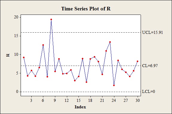
If any observation that lies outside of the control limits, then that indicates an out-of-control signal.

According to the data it is clear that range of sample above the upper control limit. Hence the process variance appears to be out of control.

By eliminating the sample 8 from the process, again inspect the observations.

The value of $\overline{X}$ and R after the elimination is:

Software procedure:

Step-by-step procedure to obtain descriptive measures of thickness using MINITAB software is as follows,

• Choose Stat > Basic Statistics > Display Descriptive Statistics.
• In Variables enter the columns X-bar and R.
• Click OK.

Output obtained using MINITAB is given below:

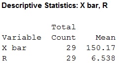
From the MINITAB, the value of $\overline{\overline{X}}=150.166$,$\overline{R}=6.538$.

The corrected control limits were given below:

Substitute $D_4$ as 2.282 and $\overline{R}$ as 6.538 in the UCL formula,

$\begin{array}{c}UCL=D_4\overline{R}\\ =2.282\left(6.538\right)\\ =14.920\end{array}$

Substitute $\overline{R}$ as 6.538,

$CL=6.538$

For $D_3$:

From Table A.10 Control chart constants,

• Locate sample size n, 4 in the first column.
• Locate the value that corresponds to the sample size 4 in column $D_3$
• The intersection value is 0.

Substitute $D_3$ as 0 and $\overline{R}$ as 6.538 in the LCL formula,

$\begin{array}{c}\text{LCL}=D_3\overline{R}\\ =0\left(6.538\right)\\ =0\end{array}$

Thus, the upper, center line and lower control limits for $\overline{R}$ chart is $\underset{\_}{\text{UCL}=14.920,CL=6.538\text{and LCL}=0}$.

R chart:

Software procedure:

Step-by-step software procedure to construct a R-chart using MINITAB software is as follows,

• Choose Stat > Time Series > Time Series Plots > Simple.
• In Series, enter columns R.
• Click OK.
• Right click on graph select Add > Reference lines.
• Enter UCL=14.920 under Show reference lines at Y values.
• Again right click on graph select Add > Reference lines.
• Enter CL=6.538 under Show reference lines at Y values.
• Similarly, enter LCL=0 under Show reference lines at Y values
• Click OK

Output obtained using MINITAB is given below:

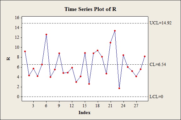
According to the data it is clear that the process variance does appears to be in control.

To determine

Obtain the $3\sigma$ control limits for $\overline{X}$ chart using sample ranges.

Check whether or not the process mean is in control, otherwise detect the sample at which the process is out of control.

Answer to Problem 12E

The upper and lower control limits for $\overline{X}$ chart is $\underset{\_}{\text{UCL}=154.932,CL=150.166\text{ and LCL}=145.400}$.

Yes, the process is in control.

Explanation of Solution

Calculation:

Control Limits For an$\overline{X}$chart:

When process mean and standard deviation are unknown is,

$\begin{array}{c}3\sigma \text{upper}\text{limit}=\overline{\overline{X}}+A_2\overline{R}\\ \text{Center}\text{line}=\overline{\overline{X}}\\ 3\sigma \text{lower}\text{limit}=\overline{\overline{X}}-A_2\overline{R}\end{array}$

Where, $\overline{R}=\frac{{\displaystyle \sum _{i=1}^N{R}_i}}{N}$ and $\overline{\overline{X}}=\frac{{\displaystyle \sum _{i=1}^N{\overline{X}}_i}}{N}$

Let N denotes the number of sample and n be the sample size.

For $A_2$:

From Table A.10 Control chart constants,

• Locate sample size n, 4 in the first column.
• Locate the value that corresponds to the sample size 4 in column $A_2$
• The intersection value is 0.729.

Substitute $A_2$ as 0.729,$\overline{\overline{X}}$ as 150.166 and $\overline{R}$ as 6.538 in the UCL formula,

$\begin{array}{c}UCL=\overline{\overline{X}}+A_2\overline{R}\\ =150.166+0.729\left(6.538\right)\\ =150.166+4.7662\\ =154.932\end{array}$

Substitute $\overline{\overline{X}}$ as 150.166,

$CL=150.166$

Substitute $A_2$ as 0.729,$\overline{\overline{X}}$ as 150.166 and $\overline{R}$ as 6.538 in the LCL formula,

$\begin{array}{c}LCL=\overline{\overline{X}}-A_2\overline{R}\\ =150.166-0.729\left(6.538\right)\\ =150.166-4.7662\\ =145.400\end{array}$

Thus, the upper and lower control limits for $\overline{X}$ chart is $\underset{\_}{\text{UCL}=154.932,CL=150.166\text{ and LCL}=145.400}$.

$\overline{X}$chart:

Software procedure:

Step-by-step software procedure to construct a $\overline{X}$-chart using MINITAB software is as follows,

• Choose Stat > Time Series > Time Series Plots > Simple.
• In Series, enter columns X-Bar.
• Click OK.
• Right click on graph select Add > Reference lines.
• Enter UCL=154.932 under Show reference lines at Y values.
• Again right click on graph select Add > Reference lines.
• Enter CL=150.166 under Show reference lines at Y values.
• Similarly, enter LCL=145.400 under Show reference lines at Y values
• Click OK

Output obtained using MINITAB is given below:

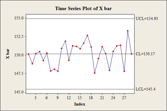
From the MINITAB output, it has been verified clearly that the process variance lies within the upper and lower control limit.

Hence the process variance is in control.

To determine

Check whether or not the process mean is in control, otherwise detect the sample at which the process is out of control based on Western Electric rules.

Answer to Problem 12E

Yes, the process is in control.

Explanation of Solution

Calculation:

Western Electric rules:

The condition which states that the process is out of control is given below:

• The point which is plotted outside the $3\sigma$ control limits.
• Out of three succeeding points, two points plotted above the upper $2\sigma$ control limits, or out of three succeeding points, two points plotted above the lower $2\sigma$ control limits.
• Out of five succeeding points, four points plotted above the upper $1\sigma$ control limits, or out of five succeeding points, four points plotted above the lower $1\sigma$ control limits.
• Finally, the eight succeeding points is to be plotted on same part of the center line.

Control Limits of an$\overline{X}$chart for $1\sigma$limit:

$\begin{array}{c}1\sigma \text{upper}\text{limit}\left(UCL\right)=\overline{\overline{X}}+A_2\frac{\overline{R}}{3}\\ \text{Center}\text{line}\left(CL\right)=\overline{\overline{X}}\\ 1\sigma \text{lower}\text{limit}\left(LCL\right)=\overline{\overline{X}}-A_2\frac{\overline{R}}{3}\end{array}$

Let N denotes the number of sample and n be the sample size.

For $A_2$:

From Table A.10 Control chart constants,

• Locate sample size n, 4 in the first column.
• Locate the value that corresponds to the sample size 4 in column $A_2$
• The intersection value is 0.729.

Substitute $A_2$ as 0.729,$\overline{\overline{X}}$ as 150.166 and $\overline{R}$ as 6.538 in the UCL formula,

$\begin{array}{c}UCL=\overline{\overline{X}}+A_2\frac{\overline{R}}{3}\\ =150.166+0.729\left(\frac{6.538}{3}\right)\\ =150.166+1.5887\\ =151.755\end{array}$

Substitute $\overline{\overline{X}}$ as 150.166,

$CL=150.166$

Substitute $A_2$ as 0.729,$\overline{\overline{X}}$ as 150.166 and $\overline{R}$ as 6.538 in the LCL formula,

$\begin{array}{c}LCL=\overline{\overline{X}}-A_2\frac{\overline{R}}{3}\\ =150.166-0.729\left(\frac{6.538}{3}\right)\\ =150.166-1.5887\\ =148.577\end{array}$

Thus, the upper, center line and lower $1\sigma$ control limits for $\overline{X}$ chart is $\underset{\_}{\text{UCL}=151.755\text{ and LCL}=148.577}$.

Control Limits of an$\overline{X}$chart for $2\sigma$limit:

$\begin{array}{c}2\sigma \text{upper}\text{limit}\left(UCL\right)=\overline{\overline{X}}+2A_2\frac{\overline{R}}{3}\\ \text{Center}\text{line}\left(CL\right)=\overline{\overline{X}}\\ 2\sigma \text{lower}\text{limit}\left(LCL\right)=\overline{\overline{X}}-2A_2\frac{\overline{R}}{3}\end{array}$

Where, $\overline{R}=\frac{{\displaystyle \sum _{i=1}^N{R}_i}}{N}$ and $\overline{\overline{X}}=\frac{{\displaystyle \sum _{i=1}^N{\overline{X}}_i}}{N}$

Substitute $A_2$ as 0.729,$\overline{\overline{X}}$ as 150.166 and $\overline{R}$ as 6.538 in the UCL formula,

$\begin{array}{c}UCL=\overline{\overline{X}}+2A_2\frac{\overline{R}}{3}\\ =150.166+2\left(0.729\right)\left(\frac{6.538}{3}\right)\\ =150.166+2\left(1.5887\right)\\ =150.166+3.1774\\ =153.343\end{array}$

Substitute $A_2$ as 0.729,$\overline{\overline{X}}$ as 150.166 and $\overline{R}$ as 6.538 in the LCL formula,

$\begin{array}{c}LCL=\overline{\overline{X}}-2A_2\frac{\overline{R}}{3}\\ =150.166-2\left(0.729\right)\left(\frac{6.538}{3}\right)\\ =150.166-2\left(1.5887\right)\\ =150.166-3.1774\\ =146.989\end{array}$

Thus, the upper, center line and lower $2\sigma$ control limits for $\overline{X}$ chart is $\underset{\_}{\text{UCL}=153.343\text{and LCL}=146.989}$.

$\overline{X}$chart for $1\sigma ,2\sigma \text{ and }3\sigma$limits:

Software procedure:

Step-by-step software procedure to construct a $\overline{X}$-chart using MINITAB software is as follows,

• Choose Stat > Time Series > Time Series Plots > Simple.
• In Series, enter columns X-Bar.
• Click OK.
• Right click on graph select Add > Reference lines.
• Enter 3 sigma UCL=154.932 under Show reference lines at Y values.
• Again right click on graph select Add > Reference lines.
• Enter CL=150.166 under Show reference lines at Y values.
• Similarly, enter 3 sigma LCL=145.400 under Show reference lines at Y values
• Enter 2 sigma UCL=153.343 under Show reference lines at Y values.
• Again right click on graph select Add > Reference lines.
• Enter 2 sigma LCL=146.989 under Show reference lines at Y values.
• Again right click on graph select Add > Reference lines.
• Enter 1 sigma UCL=151.755 under Show reference lines at Y values.
• Similarly, enter 1 sigma LCL=148.577 under Show reference lines at Y values
• Click OK

Output obtained using MINITAB is given below:

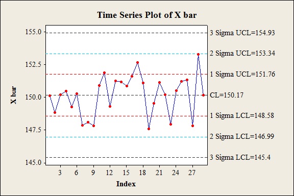
From the MINITAB output, it has been verified clearly that the process variance is in control.

Based on the condition of Western Electric rules, the sample 8 of the sample mean does not falls within the upper control limit and lower control limit for first time and it has be eliminated in part (a).

The recomputed plot fall with the upper and lower control limit.

Thus, the process is in control.