
Concept explainers
Videos
Instructions: You may use Excel, MegaStat, Minitab, JMP, or another computer package of your choice. Attach appropriate copies of the output or capture the screens, tables, and relevant graphs and include them in a written report. Try to state your conclusions succinctly in language that would be clear to a decision maker who is a nonstatistician. Exercises marked * are based on optional material. Answer the following questions, or those your instructor assigns.
- a. Choose an appropriate ANOVA model. State the hypotheses to be tested.
- b. Display the data visually (e.g., dot plots or line plots by factor). What do the displays show?
- c. Do the ANOVA calculations using the computer.
- d. State the decision rule for α = .05 and make the decision. Interpret the p-value.
- e. In your judgment, are the observed differences in treatment means (if any) large enough to be of practical importance?
- f. Given the nature of the data, would more data collection be practical?
- g. Perform Tukey multiple comparison tests and discuss the results.
- h. Perform a test for homogeneity of variances. Explain fully.
Below are data on truck production (number of vehicles completed) during the second shift at five truck plants for each day in a randomly chosen week. Research question: Are the mean production rates the same by plant and by day?

a.
Choose appropriate ANOVA model. State the hypothesis.
Answer to Problem 43CE
Two-factor ANOVA without replication is used in this situation.
For factor A:
Null hypothesis:
Alternative hypothesis:
For factor B:
Null hypothesis:
Alternative hypothesis:
Explanation of Solution
The given information is a production rate for three plants.
Two-factor ANOVA without replication is mainly used for comparing effect of two factors without testing the interaction. Therefore, the data comparison of effect of two factors can be model using two-factor ANOVA without replication.
Factor A denotes the plant and B denotes the day.
State the hypotheses:
For factor A:
Null hypothesis:
There is no effect for plant.
Alternative hypothesis:
At least one plant has effect.
For factor B:
Null hypothesis:
There is no effect for day.
Alternative hypothesis:
At least one day has effect.
b.
Display the data for each plot and explain the plot.
Answer to Problem 43CE
The dot plot is given by:

Explanation of Solution
Calculation:
Dot plot:
Software procedure:
Step-by-step procedure for Dot plot using the Mega Stat is given below:
- • Open an EXCEL file.
- • In Mega Stat, select Analysis of variance and then Randomized block ANOVA.
- • In Input range drop down box, select Values.
- • Click on Plot the data.
- • Click OK.
The output using the Mega Stat software is given below:
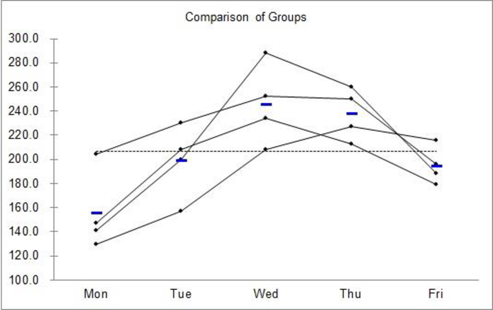
Observations:
From the dot plot it is clear that mean production rate for Wednesday and Thursday. That is, the mean production rates are different. Therefore, mean production rate for different days are significant.
c.
Perform ANOVA.
Explanation of Solution
Calculation:
Two-factor ANOVA without replication and Turkey’s comparison:
Software procedure:
Step-by-step procedure for Two-factor ANOVA without replication and Turkey’s comparison using the MegaStat is given below:
- • Open an EXCEL file.
- • In Mega Stat, select Analysis of variance and then Randomized block ANOVA.
- • In Input range drop down box, select Values.
- • In post-hoc analysis select p less than 0.05
- • Click OK.
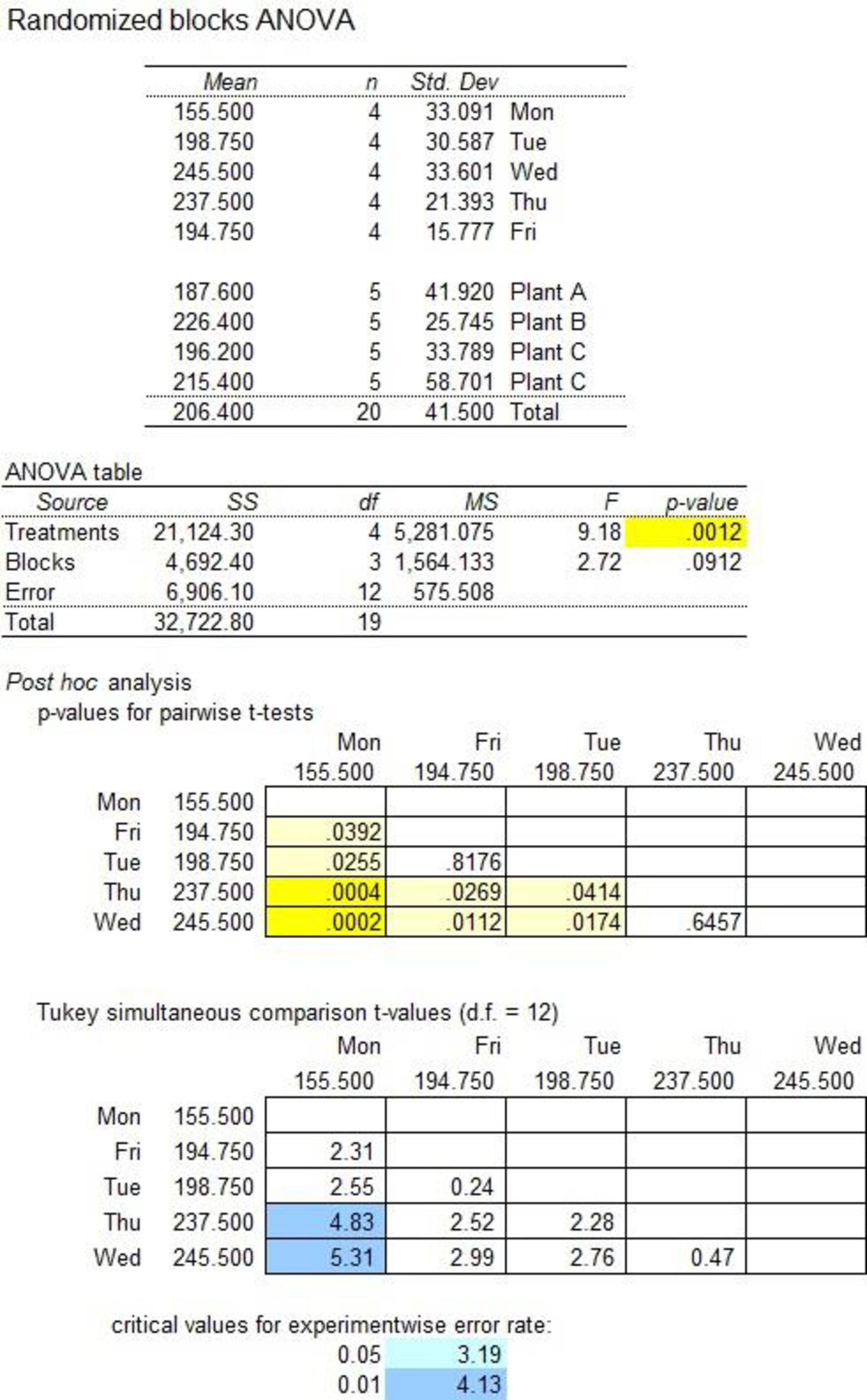
The output using the Mega Stat software is given below:
d.
Explain the conclusion.
Interpret the p-value.
Answer to Problem 43CE
There is enough evidence to conclude that mean production rate is affected by factor day.
Explanation of Solution
Calculation:
From the MegaStat output of part (c),
The p-value for plant is 0.0912.
The p-value for factor days is 0.0012.
Rejection rule:
If
Conclusion:
For factor day:
From the MegaStat output, the p-value is 0.0012.
That is less than the significance level
That is,
Therefore, the null hypothesis is rejected.
Hence, mean production rate is affected by factor day.
For factor plant:
From the MegaStat output, the p-value is 0.0912.
That is greater than the significance level
That is,
Therefore, the null hypothesis is not rejected.
Hence, mean production rate is affected by factor plant.
Here, the p-values for day is very small. Therefore, samples were support the rejection of the null hypotheses. The p-values for plant are not very small. Therefore, samples were not support the rejection of the null hypotheses.
e.
Check whether the observed difference in treatment means large enough to be of practical importance.
Answer to Problem 43CE
The observed difference in treatment means large enough to be of practical importance.
Explanation of Solution
From the dot plot or the individual value plot it clear that mean stopping time is affected by factor days. That is factor days condition is significant. For manufacturer the production rate is important. Therefore, observed difference in treatment means large enough to be of practical importance.
f.
Check whether more data collection is practical if nature of the data is given.
Explanation of Solution
Answer will vary. One of the possible answers is given below:
The samples are taken from the Ford trucks. If the nature of the data is given then it is easy to collect samples from more trucks. Thus, the data collection is practical if nature of the data is given.
g.
Perform Turkeys test using explain the results.
Answer to Problem 43CE
There is enough evidence to conclude that significant difference among all pair of days excluding ‘Thursday and Wednesday’ and ‘Friday and Tuesday’.
Explanation of Solution
Calculation:
Significance level is
State the hypotheses:
Null hypothesis:
That is, all the pair treatment means are equal.
Alternative hypothesis:
That is, at least one pair of treatment means differ.
Here, the Turkey’s test statistic is
Rejection rule:
If
From the MegaStat output in part (c),
The value of the p-value for Monday and Friday is 0.0392.
The value of the p-value for Monday and Tuesday is 0.0255.
The value of the p-value for Monday and Thursday is 0.0004.
The value of the p-value for Monday and Wednesday is 0.0002.
The value of the p-value for Friday and Tuesday is 0.8176.
The value of the p-value for Friday and Thursday is 0.0269.
The value of the p-value for Friday and Wednesday is 0.0112.
The value of the p-value for Tuesday and Thursday is 0.0414.
The value of the p-value for Tuesday and Wednesday is 0.0174.
The value of the p-value for Thursday and Wednesday is 0.6457.
Conclusion:
For Monday and Friday:
The p-value is 0.0392, which less than the significance level is
That is,
Thus, there is enough evidence to conclude that there is significant difference among means of Monday and Friday.
For Monday and Tuesday:
The p-value is 0.0255, which less than the significance level is
That is,
Thus, there is enough evidence to conclude that there is significant difference among means of Monday and Tuesday.
For Monday and Thursday:
The p-value is 0.0004, which less than the significance level is
That is,
Thus, there is enough evidence to conclude that there is significant difference among means of Monday and Thursday.
For Monday and Wednesday:
The p-value is 0.0002, which less than the significance level is
That is,
Thus, there is enough evidence to conclude that there is significant difference among means of Monday and Wednesday.
For Friday and Tuesday:
The p-value is 0.8176, which greater than the significance level is
That is,
Thus, there is enough evidence to conclude that there no significant difference among means of Friday and Tuesday.
For Friday and Thursday:
The p-value is 0.0269, which less than the significance level is
That is,
Thus, there is enough evidence to conclude that there significant difference among means of Friday and Thursday.
For Friday and Wednesday:
The p-value is 0.0112, which less than the significance level is
That is,
Thus, there is enough evidence to conclude that there significant difference among means of Friday and Wednesday.
For Tuesday and Thursday:
The p-value is 0.0414, which less than the significance level is
That is,
Thus, there is enough evidence to conclude that there significant difference among means of Tuesday and Thursday.
For Tuesday and Wednesday:
The p-value is 0.0174, which less than the significance level is
That is,
Thus, there is enough evidence to conclude that there significant difference among means of Tuesday and Wednesday.
For Thursday and Wednesday:
The p-value is 0.6457, which greater than the significance level is
That is,
Thus, there is enough evidence to conclude that there no significant difference among means of Thursday and Wednesday.
h.
Perform test of homogeneity of variance and explain the results.
Answer to Problem 43CE
There is enough evidence to conclude that variances for days are not different.
Explanation of Solution
Calculation:
State the hypotheses:
For factor days:
Null hypothesis:
All the surface variances are equal.
Alternative hypothesis:
At least one pair of variance differs.
Rejection rule:
If
Test statistics:
The Hartley’s test statistics H is given by:
Where,
Degrees of freedom:
For between group:
Here, there are 5 days. That is
Therefore,
Thus, between group degrees of freedom are 5.
For within group:
Substitute
Therefore,
Thus, within group degrees of freedom are 3.
Critical-value:
Procedure for the value of Hartley’s H using Table 11.5:
- • Go through the row corresponding to 5 in Table 11.5 of five percent critical values of Hartley’s
- • Go through the row corresponding to 5 and column corresponding to the number of groups 3.
- • Obtain the value corresponding to (5, 3) from the table.
Thus, the critical-value is 50.7.
For surface:
The sample variances for surface are:
Here,
Substitute these values in the above equation.
Therefore,
Thus, the Hartley’s test statistics is 4.5358.
Conclusion:
Here, the H-test statistic is 4.5358.
Here,
That is test statistic is less than the critical value.
Therefore, the null hypothesis is not rejected.
Thus, there is enough evidence to conclude that variances for days are not different.
Want to see more full solutions like this?
Chapter 11 Solutions
Applied Statistics in Business and Economics with Connect Access Card with LearnSmart


- Name the four characteristics of a good definition.arrow_forwardAnswer the following questions. 5. What is the term for the arrangement that selects r objects from a set of ii objects when the order of the r objects is not important? What is the formula for calculating the number of possible outcomes for this type of arrangement?arrow_forward

 Elementary Geometry For College Students, 7eGeometryISBN:9781337614085Author:Alexander, Daniel C.; Koeberlein, Geralyn M.Publisher:Cengage,
 Big Ideas Math A Bridge To Success Algebra 1: Stu...AlgebraISBN:9781680331141Author:HOUGHTON MIFFLIN HARCOURTPublisher:Houghton Mifflin Harcourt