Elementary Statistics: A Step By Step Approach
10th Edition
ISBN: 9781259755330
Author: Allan G. Bluman
Publisher: McGraw-Hill Education
bartleby

Concept explainers

bartleby

Videos

Textbook Question
Book Icon
Chapter 12.2, Problem 8E

For Exercises 3 through 8, the null hypothesis was rejected. Use the Scheffe test when sample sizes are unequal or the Tukey test when sample sizes are equal, to test the differences between the pairs of means. Assume all variables are normally distributed, samples are independent, and the population variances are equal.

8. Exercise 20 in Section 12-1.

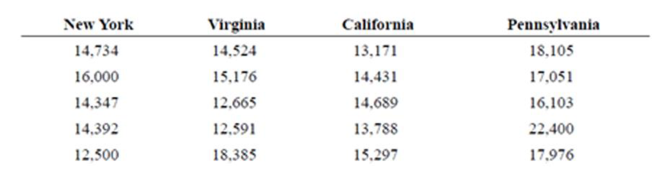
20. Average Debt of College Graduates Kiplinger’s listed the top 100 public colleges based on many factors. From that list, here is the average debt at graduation for various schools in four selected states. At a = 0.05, can it be concluded that the average debt at graduation differs for these four states?

Chapter 12.2, Problem 8E, For Exercises 3 through 8, the null hypothesis was rejected. Use the Scheffe test when sample sizes

Source: www.Kiplinger.com

Expert Solution & Answer
Check Mark
To determine

To test: The difference between the means.

Answer to Problem 8E

There is significant difference between the means X¯1 and X¯4 , X¯2 and X¯4 , and X¯3 and X¯4 .

Explanation of Solution

Given info:

The table shows the average debt at graduation for various schools in four selected states. The level of significance is 0.05.

Calculation:

Consider, X¯1 , X¯2 , X¯3 and X¯4 represents the means of New York, Virginia, California and Pennsylvania, s12,s22s32 and s42 represents the variances of samples of New York, Virginia, California and Pennsylvania.

Step-by-step procedure to obtain the test mean and standard deviation using the MINITAB software:

  • Choose Stat > Basic Statistics > Display Descriptive Statistics.
  • In Variables enter the columns New York, Virginia, California and Pennsylvania.
  • Choose option statistics, and select Mean, Variance and N total.
  • Click OK.

Output using the MINITAB software is given below:
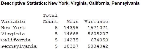
Elementary Statistics: A Step By Step Approach, Chapter 12.2, Problem 8E

The sample sizes n1,n2,n3 and n4 are 5, 5, 5 and 5.

The means are X¯1,X¯2 and X¯3 are 14395, 14668, 14275 and 18327.

The sample variances are s12,s22s32 and s42 are 1571071, 5605207, 674050 and 5834042.

Here, the samples of sizes of four states are equal. So, the test used here is Tukey test.

Tukey test:

Critical value:

Here, k is 4 and degrees of freedom v=Nk ,

Where,

N=n1+n2+n3+n4=5+5+5+5=20

Substitute 20 for N and 4 for k in v

v=Nk=204=16

The critical F-value is obtained using the Table N: Critical Values for the Tukey test with the level of significance α=0.05 .

Procedure:

  • Locate 16 in the column of v of the Table H.
  • Obtain the value in the corresponding row below 4.

That is, the critical value is 4.05.

Comparison of the means:

The formula for finding sW2 is,

sW2=(ni1)si2(ni1)

That is,

sW2=(51)1,571,071+(51)5,605,207+(51)674,050+(51)5,834,042(51)+(51)+(51)+(51)=6,284,284+22,420,828+2,696,200+23,336,16816=54,737,48016=3,421,093

Comparison between the means X¯1 and X¯2 :

The hypotheses are given below:

Null hypothesis:

H0: There is no significant difference between X¯1 and X¯2 .

Alternative hypothesis:

H1: There is significant difference between X¯1 and X¯2 .

Rejection region:

The null hypothesis would be rejected if absolute value greater than the critical value.

Absolute value:

The formula for comparing the means X¯1 and X¯2 is,

q1=X¯1X¯2sW2n

Substitute 14,395, 14,668 for X¯1 and X¯2 and 3,421,093 for sW2

q1=14,39514,6683,421,0935=273684,218.6=273827.1751=0.33

Thus, the value of q1 is –0.33.

Hence, the absolute value of q1 is 0.33.

Conclusion:

The absolute value is 0.33.

Here, the absolute value is lesser than the critical value.

That is, 0.33<4.05 .

Thus, the null hypothesis is not rejected.

Hence, there is no significant difference between the means X¯1 and X¯2 .

Comparison between the means X¯1 and X¯3 :

The hypotheses are given below:

Null hypothesis:

H0: There is no significant difference between X¯1 and X¯3 .

Alternative hypothesis:

H1: There is significant difference between X¯1 and X¯3 .

Rejection region:

The null hypothesis would be rejected if absolute value greater than the critical value.

Absolute value:

The formula for comparing the means X¯1 and X¯3 is,

q2=X¯1X¯3sW2n

Substitute 14,395, 14,275 for X¯1 and X¯3 and 3,421,093 for sW2

q2=14,39514,2753,421,0935=120684,218.6=120827.1751=0.15

Thus, the value of q2 is 0.15.

Hence, the absolute value of q2 is 0.15.

Conclusion:

The absolute value is 0.15.

Here, the absolute value is lesser than the critical value.

That is, 0.15<4.05 .

Thus, the null hypothesis is not rejected.

Hence, there is no significant difference between the means X¯1 and X¯3 .

Comparison between the means X¯1 and X¯4 :

The hypotheses are given below:

Null hypothesis:

H0: There is no significant difference between X¯1 and X¯4 .

Alternative hypothesis:

H1: There is significant difference between X¯1 and X¯4 .

Rejection region:

The null hypothesis would be rejected if absolute value greater than the critical value.

Absolute value:

The formula for comparing the means X¯1 and X¯4 is,

q3=X¯1X¯4sW2n

Substitute 14,395, 18,327 for X¯1 and X¯4 and 3,421,093 for sW2

q3=14,39518,3273,421,0935=3932684,218.6=3932827.1751=4.75

Thus, the value of q3 is –4.75.

Hence, the absolute value of q3 is 4.75.

Conclusion:

The absolute value is 4.75.

Here, the absolute value is greater than the critical value.

That is, 4.75>4.05 .

Thus, the null hypothesis is rejected.

Hence, there is significant difference between the means X¯1 and X¯4 .

Comparison between the means X¯2 and X¯3 :

The hypotheses are given below:

Null hypothesis:

H0: There is no significant difference between X¯2 and X¯3 .

Alternative hypothesis:

H1: There is significant difference between X¯2 and X¯3 .

Rejection region:

The null hypothesis would be rejected if absolute value greater than the critical value.

Absolute value:

The formula for comparing the means X¯2 and X¯3 is,

q4=X¯2X¯3sW2n

Substitute 14,668 and 14,275 for X¯2 and X¯3 and 3,421,093 for sW2

q4=14,66814,2753,421,0935=393684,218.6=393827.1751=0.48

Thus, the value of q4 is 0.48.

Hence, the absolute value of q4 is 0.48.

Conclusion:

The absolute value is 0.48.

Here, the absolute value is lesser than the critical value.

That is, 0.48<4.05 .

Thus, the null hypothesis is rejected.

Hence, there is no significant difference between the means X¯2 and X¯3 .

Comparison between the means X¯2 and X¯4 :

The hypotheses are given below:

Null hypothesis:

H0: There is no significant difference between X¯2 and X¯4 .

Alternative hypothesis:

H1: There is significant difference between X¯2 and X¯4 .

Rejection region:

The null hypothesis would be rejected if absolute value greater than the critical value.

Absolute value:

The formula for comparing the means X¯2 and X¯4 is,

q5=X¯2X¯4sW2n

Substitute 14,668 and 18,327 for X¯2 and X¯4 and 3,421,093 for sW2

q5=14,66818,3273,421,0935=3659684,218.6=3659827.1751=4.42

Thus, the value of q5 is –4.42.

Hence, the absolute value of q5 is 4.42.

Conclusion:

The absolute value is 4.42.

Here, the absolute value is greater than the critical value.

That is, 4.42>4.05 .

Thus, the null hypothesis is rejected.

Hence, there is significant difference between the means X¯2 and X¯4 .

Comparison between the means X¯3 and X¯4 :

The hypotheses are given below:

Null hypothesis:

H0: There is no significant difference between X¯3 and X¯4 .

Alternative hypothesis:

H1: There is significant difference between X¯3 and X¯4 .

Rejection region:

The null hypothesis would be rejected if absolute value greater than the critical value.

Absolute value:

The formula for comparing the means X¯3 and X¯4 is,

q5=X¯3X¯4sW2n

Substitute 14,275 and 18,327 for X¯3 and X¯4 and 3,421,093 for sW2

q6=14,27518,3273,421,0935=4052684,218.6=4052827.1751=4.90

Thus, the value of q6 is –4.90.

Hence, the absolute value of q6 is 4.90.

Conclusion:

The absolute value is 4.90.

Here, the absolute value is greater than the critical value.

That is, 4.90>4.05 .

Thus, the null hypothesis is rejected.

Hence, there is significant difference between the means X¯3 and X¯4 .

Justification:

Here, there is significant difference between the means X¯1 and X¯4 , X¯2 and X¯4 , and X¯3 and X¯4 .

Want to see more full solutions like this?

Subscribe now to access step-by-step solutions to millions of textbook problems written by subject matter experts!

Chapter 12 Solutions

Elementary Statistics: A Step By Step Approach

Ch. 12.1 - For Exercises 7 through 20, assume that all...Ch. 12.1 - Prob. 11ECh. 12.1 - For Exercises 7 through 20, assume that all...Ch. 12.1 - For Exercises 7 through 20, assume that all...Ch. 12.1 - For Exercises 7 through 20, assume that all...Ch. 12.1 - Prob. 15ECh. 12.1 - For Exercises 7 through 20, assume that all...Ch. 12.1 - For Exercises 7 through 20, assume that all...Ch. 12.1 - For Exercises 7 through 20, assume that all...Ch. 12.1 - For Exercises 7 through 20, assume that all...Ch. 12.1 - For Exercises 7 through 20, assume that all...Ch. 12.2 - Colors That Make You Smarter The following set of...Ch. 12.2 - What two tests can be used to compare two means...Ch. 12.2 - Explain the difference between the two tests used...Ch. 12.2 - For Exercises 3 through 8, the null hypothesis was...Ch. 12.2 - For Exercises 3 through 8, the null hypothesis was...Ch. 12.2 - For Exercises 3 through 8, the null hypothesis was...Ch. 12.2 - For Exercises 3 through 8, the null hypothesis was...Ch. 12.2 - For Exercises 3 through 8, the null hypothesis was...Ch. 12.2 - For Exercises 3 through 8, the null hypothesis was...Ch. 12.2 - For Exercises 9 through 13, do a complete one-way...Ch. 12.2 - Prob. 10ECh. 12.2 - For Exercises 9 through 13, do a complete one-way...Ch. 12.2 - For Exercises 9 through 13, do a complete one-way...Ch. 12.2 - Prob. 13ECh. 12.2 - Prob. 14ECh. 12.3 - Automobile Sales Techniques The following outputs...Ch. 12.3 - Prob. 1ECh. 12.3 - Explain what is meant by main effects and...Ch. 12.3 - Prob. 3ECh. 12.3 - How are the F test values computed?Ch. 12.3 - Prob. 5ECh. 12.3 - In a two-way ANOVA, variable A has six levels and...Ch. 12.3 - Prob. 7ECh. 12.3 - When can the main effects for the two-way ANOVA be...Ch. 12.3 - Prob. 9ECh. 12.3 - For Exercises 9 through 15, perform these steps....Ch. 12.3 - For Exercises 9 through 15, perform these steps....Ch. 12.3 - For Exercises 9 through 15, perform these steps....Ch. 12.3 - Prob. 13ECh. 12.3 - For Exercises 9 through 15, perform these steps....Ch. 12.3 - Prob. 15ECh. 12 - If the null hypothesis is rejected in Exercises 1...Ch. 12 - Prob. 12.1.2RECh. 12 - Prob. 12.1.3RECh. 12 - Prob. 12.1.4RECh. 12 - Prob. 12.1.5RECh. 12 - If the null hypothesis is rejected in Exercises 1...Ch. 12 - Prob. 12.1.7RECh. 12 - Prob. 12.1.8RECh. 12 - Review Preparation for Statistics A statistics...Ch. 12 - Effects of Different Types of Diets A medical...Ch. 12 - Prob. 1DACh. 12 - Prob. 2DACh. 12 - Prob. 3DACh. 12 - Prob. 1CQCh. 12 - Prob. 2CQCh. 12 - Prob. 3CQCh. 12 - Determine whether each statement is true or false....Ch. 12 - Prob. 5CQCh. 12 - Prob. 6CQCh. 12 - Prob. 7CQCh. 12 - Prob. 8CQCh. 12 - Complete the following statements with the best...Ch. 12 - Prob. 10CQCh. 12 - For Exercises 11 through 17, use the traditional...Ch. 12 - Prob. 12CQCh. 12 - Prob. 13CQCh. 12 - Prob. 14CQCh. 12 - Prob. 15CQCh. 12 - Prob. 16CQCh. 12 - For Exercises 11 through 17, use the traditional...Ch. 12 - Shown here are the abstract and two tables from a...Ch. 12 - Shown here are the abstract and two tables from a...Ch. 12 - Prob. 3CTCCh. 12 - Prob. 4CTCCh. 12 - Prob. 5CTCCh. 12 - Prob. 6CTCCh. 12 - Prob. 7CTCCh. 12 - Adult Children of Alcoholics Shown here are the...Ch. 12 - Prob. 9CTCCh. 12 - Prob. 10CTCCh. 12 - Prob. 11CTC
Knowledge Booster
Background pattern image
Statistics
Learn more about
Need a deep-dive on the concept behind this application? Look no further. Learn more about this topic, statistics and related others by exploring similar questions and additional content below.
Recommended textbooks for you
Text book image
Glencoe Algebra 1, Student Edition, 9780079039897...
Algebra
ISBN:9780079039897
Author:Carter
Publisher:McGraw Hill
Statistics 4.1 Point Estimators; Author: Dr. Jack L. Jackson II;https://www.youtube.com/watch?v=2MrI0J8XCEE;License: Standard YouTube License, CC-BY
Statistics 101: Point Estimators; Author: Brandon Foltz;https://www.youtube.com/watch?v=4v41z3HwLaM;License: Standard YouTube License, CC-BY
Central limit theorem; Author: 365 Data Science;https://www.youtube.com/watch?v=b5xQmk9veZ4;License: Standard YouTube License, CC-BY
Point Estimate Definition & Example; Author: Prof. Essa;https://www.youtube.com/watch?v=OTVwtvQmSn0;License: Standard Youtube License
Point Estimation; Author: Vamsidhar Ambatipudi;https://www.youtube.com/watch?v=flqhlM2bZWc;License: Standard Youtube License