6th Edition

ISBN: 9781259957598

Author: DOANE

Publisher: RENT MCG

Concept explainers

Correlation defines a relationship between two independent variables. It tells the degree to which variables move in relation to each other. When two sets of data are related to each other, there is a correlation between them.

Linear Correlation

A correlation is used to determine the relationships between numerical and categorical variables. In other words, it is an indicator of how things are connected to one another. The correlation analysis is the study of how variables are related.

Regression Analysis

Regression analysis is a statistical method in which it estimates the relationship between a dependent variable and one or more independent variable. In simple terms dependent variable is called as outcome variable and independent variable is called as p…

Videos

Textbook Question

Chapter 12.6, Problem 27SE

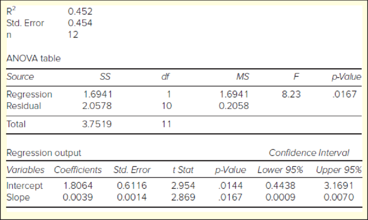
Below is a regression using X = home price (000), Y = annual taxes (000), n = 20 homes. (a) Write the fitted regression equation. (b) Write the formula for each t statistic and verify the t statistics shown below. (c) State the degrees of freedom for the t tests and find the two-tail critical value for t using Excel. (d) Use Excel’s function =T.DIST.2T(t, d.f.) to verify the p-value shown for each t statistic (slope, intercept). (e) Verify that F = t² for the slope. (f) In your own words, describe the fit of this regression.

Chapter 12.6, Problem 27SE, Below is a regression using X = home price (000), Y = annual taxes (000), n = 20 homes. (a) Write

Expert Solution & Answer

Want to see the full answer?

Check out a sample textbook solution

See solution

Chapter 12.5, Problem 26SE

Chapter 12.6, Problem 28SE

Students have asked these similar questions

The following estimated regression model was developed relating yearly income (y in $1000s) of 30 individuals with their age (x1) and their gender (x2) (0 if male and 1 if female).ŷ = 30 + 0.7x1 + 3x2Also provided are SST = 1200 and SSE = 384.The yearly income of a 24-year-old female individual is _____.

You have obtained a sub-sample of 1744 individuals from the Current Population Survey (CPS) and are interested in the relationship between weekly earnings and age. The regression, using heteroskedasticity-robust standard errors, yielded the following result: = 239.16 + 3.75× Age, R2 = 0.15, SER = 287.21., where Earn and Age are measured in dollars and years respectively. Interpret the intercept? Interpret the slope coefficient b) Is the effect of age on earnings large? The average age in this sample is 37.5 years. What is annual income in the sample? (e) Interpret the measures of fit.

The birth lengths in cm (x) and birth weights in kg (y) of a sample of 50 newborn female babies are compared, yielding a correlation coefficient of r=0.578 and a linear regression equation of ŷ =−8.89+0.243x The babies all had lengths between 46.5 and 53.0 cm, and weights between 2.50 and 4.05 kg. Based on this, predict the birth weight of a newborn female baby with a birth length of 48.5 cm.

Chapter 12 Solutions

APPLIED STAT.IN BUS.+ECONOMICS

Ch. 12.1 - For each sample, do a test for zero correlation....Ch. 12.1 - Instructions for Exercises 12.2 and 12.3: (a) Make...Ch. 12.1 - Prob. 3SE Ch. 12.1 - Prob. 4SE Ch. 12.1 - Instructions for exercises 12.412.6: (a) Make a...Ch. 12.1 - Prob. 6SE Ch. 12.2 - (a) Interpret the slope of the fitted regression...Ch. 12.2 - (a) Interpret the slope of the fitted regression...Ch. 12.2 - Prob. 9SE Ch. 12.2 - (a) Interpret the slope of the fitted regression...

Knowledge Booster

$Statistics$

Learn more about

Need a deep-dive on the concept behind this application? Look no further. Learn more about this topic, statistics and related others by exploring similar questions and additional content below.