Chapter 14, Problem 31P

a)

Summary Introduction

To estimate: The regression equation.

Introduction: Forecasting is a technique of predicting future events based on historical data and projecting them into the future with a mathematical model. Forecasting may be an intuitive or subjective prediction.

Explanation of Solution

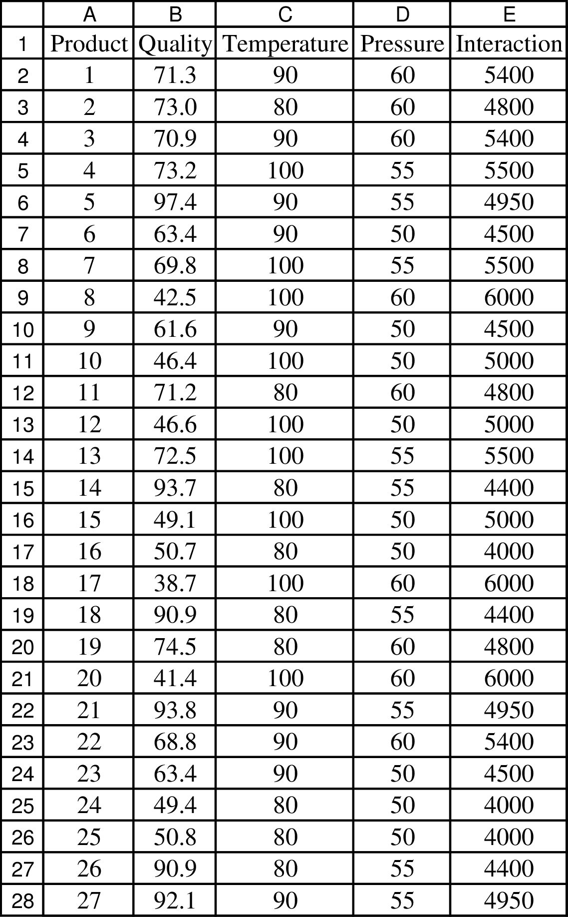
Data:

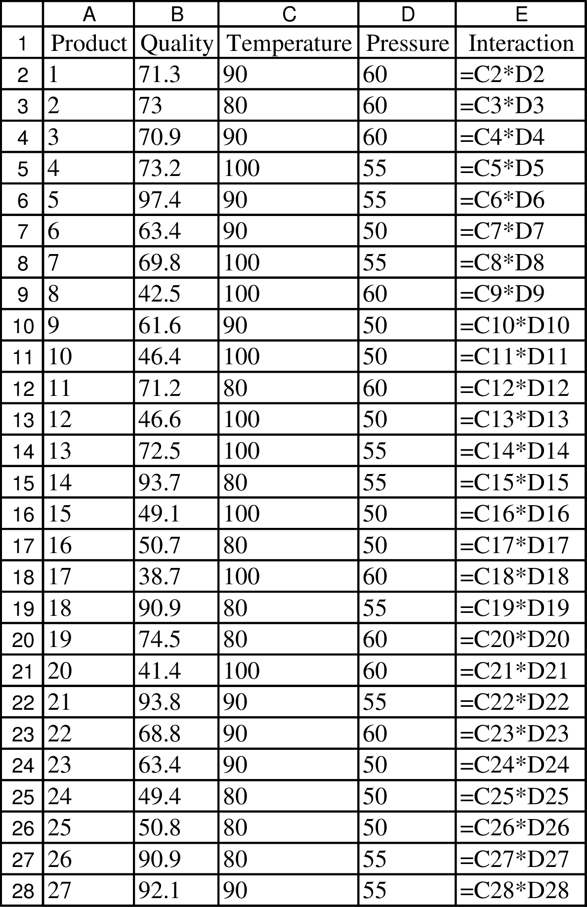
Formulae to determine the data:

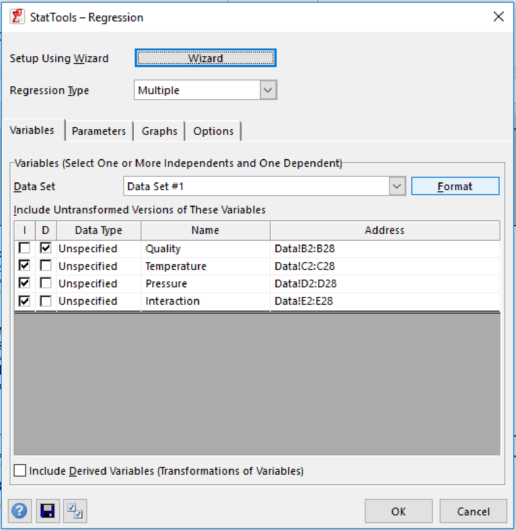
Regression using StatTools:

Regression and classification from the StatTools should be used. The below image shows the regression parameter table from StatTools:

Regression result:

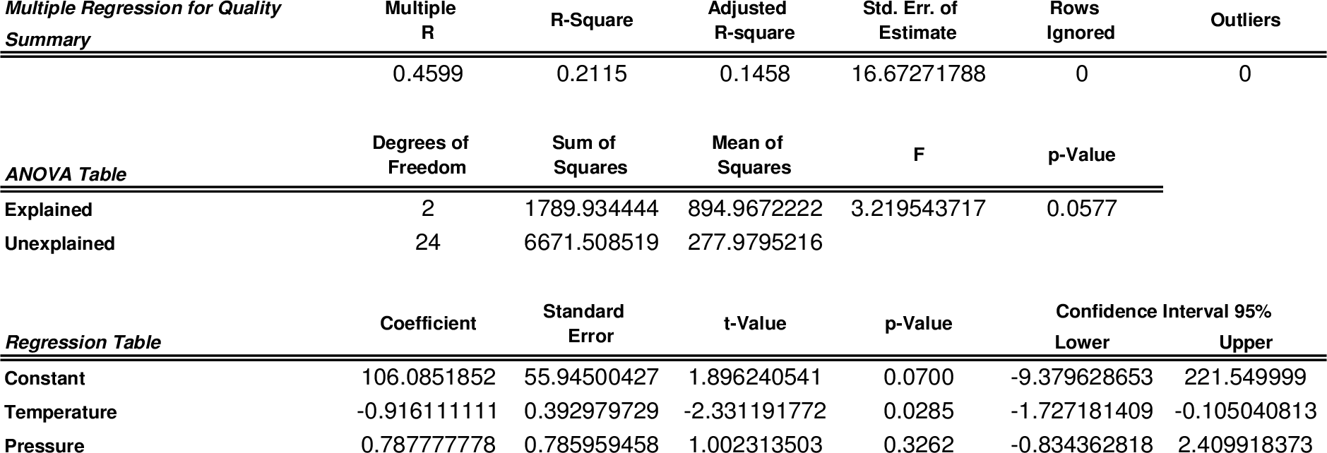
Hence, the regression equation is Quality = 106.085 – 0.916 temperature + 0.788 pressure. The value of R-square is 0.2115. The quality score falls by 0.916 and the pressure would remain constant when the temperature increases by one degree. The quality score rises by 0.788 and the temperature would remain constant when the pressure increases by one pound.

b)

Summary Introduction

To run: The regression by adding an interaction term between pressure and temperature.

Introduction: Forecasting is a technique of predicting future events based on historical data and projecting them into the future with a mathematical model. Forecasting may be an intuitive or subjective prediction.

Explanation of Solution

Data:

Formulae to determine the data:

Regression using StatTools:

Regression and classification from the StatTools should be used. The below image shows the regression parameter table from StatTools:

Regression result:

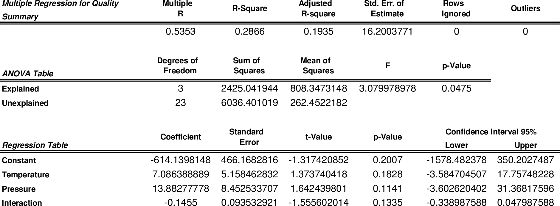
The above table provides the estimated coefficients. The standard error of estimate falls and the adjusted R-square rises.

c)

Summary Introduction

To determine: The difference between the estimated coefficients in the two equations.

Introduction: Forecasting is a technique of predicting future events based on historical data and projecting them into the future with a mathematical model. Forecasting may be an intuitive or subjective prediction.

Explanation of Solution

The quality score would increase by 7.086 – 0.145×pressure and the pressure would remain constant when the temperature increases by one degree. The quality score would increase by 13.883 – 0.145×temperature and the temperature would remain constant when the pressure increases by one pound per square inch. Based on the level of the pressure, the coefficient would indicate the quality change rate with respect to the temperature.