
Concept explainers
Videos
The Professional Golfers Association (PGA) maintains data on performance and earnings for members of the PGA Tour. For the 2012 season Bubba Watson led all players in total driving distance, with an average of 309.2 yards per drive. Some of the factors thought to influence driving distance are club head speed, ball speed, and launch angle. For the 2012 season Bubba Watson had an average club head speed of 124.69 miles per hour, an average ball speed of 184.98 miles per hour, and an average launch angle of 8.79 degrees. The DATAfile named PGADrivingDist contains data on total driving distance and the factors related to driving distance for 190 members of the PGA Tour (PGA Tour website, November 1, 2012). Descriptions for the variables in the data set follow.
Club Head Speed: Speed at which the club impacts the ball (mph).
Ball Speed: Peak speed of the golf ball at launch (mph).
Launch Angle: Vertical launch angle of the ball immediately after leaving the club (degrees).
Total Distance: The average number of yards per drive.
- a. Develop an estimated regression equation that can be used to predict the average number of yards per drive given the club head speed.
- b. Develop an estimated regression equation that can be used to predict the average number of yards per drive given the ball speed.
- c. A recommendation has been made to develop an estimated regression equation that uses both club head speed and ball speed to predict the average number of yards per drive. Do you agree with this? Explain.
- d. Develop an estimated regression equation that can be used to predict the average number of yards per drive given the ball speed and the launch angle.
- e. Suppose a new member of the PGA Tour for 2013 has a ball speed of 170 miles per hour and a launch angle of 11 degrees. Use the estimated regression equation in part (d) to predict the average number of yards per drive for this player.
a.
Find the estimated regression equation that could be used to predict the average number of yards per drive given the club head speed.
Answer to Problem 9E
The estimated regression equation that could be used to predict the average number of yards per drive given the club head speed is
Explanation of Solution
Calculation:
The Professional Golfers Association (PGA) data consist of information regarding to the speed at which the club impacts the ball (club head speed), peak speed of the golf ball at launch (ball speed), vertical launch angle of the ball immediately after leaving the club (launch angle), and the average number of yards per drive (total distance).
Multiple linear regression model:
A multiple linear regression model is given as
Denote y as the dependent variable total distance.
Regression:
Software procedure:
Step-by-step procedure to get regression equation using EXCEL software:
- Open the file PGADrivingDist.
- Select Data > Data Analysis > Regression.
- Click OK.
- Under Input Y Range enter $E$1:$E$191.
- Under Input X Range enter $B$1:$B$191.
- Click the box of Labels.
- Under Output Range enter $H$1.
- Click OK.
Output obtained using EXCEL software is given as follows:
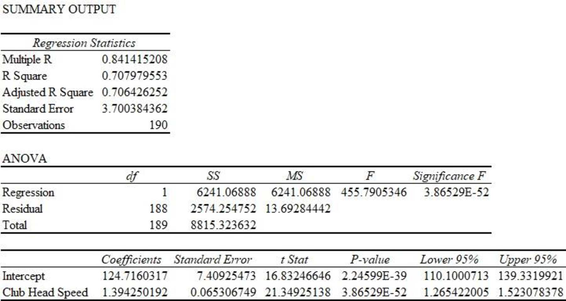
Thus, the estimated regression equation that could be used to predict the average number of yards per drive given the club head speed is
b.
Find the estimated regression equation that could be used to predict the average number of yards per drive given the ball speed.
Answer to Problem 9E
The estimated regression equation that could be used to predict the average number of yards per drive given the ball speed is
Explanation of Solution
Calculation:
The regression equation can be obtained using excel software.
Regression:
Software procedure:
Step-by-step procedure to get the regression equation using EXCEL software:
- Open the file PGADrivingDist.
- Select Data > Data Analysis > Regression.
- Click OK.
- Under Input Y Range enter $E$1:$E$191.
- Under Input X Range enter $C$1:$C$191.
- Click the box of Labels.
- Under Output Range enter $H$24.
- Click OK.
Output obtained using EXCEL software is given as follows:
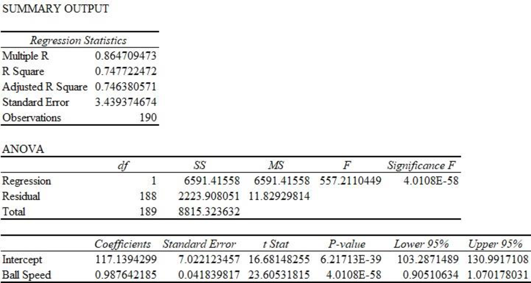
Thus, the estimated regression equation that could be used to predict the average number of yards per drive given the ball speed is
c.
Explain whether developing an estimated regression equation that uses both club head speed and ball speed to predict the average number of yards per drive is useful or not.
Explanation of Solution
Calculation:
Regression:
Software procedure:
Step-by-step procedure to get the regression equation using EXCEL software:
- Open the file PGADrivingDist.
- Select Data > Data Analysis > Regression.
- Click OK.
- Under Input Y Range enter $E$1:$E$191.
- Under Input X Range enter $B$1:$C$191.
- Click the box of Labels.
- Under Output Range enter $H$24.
- Click OK.
Output obtained using EXCEL software is given as follows:
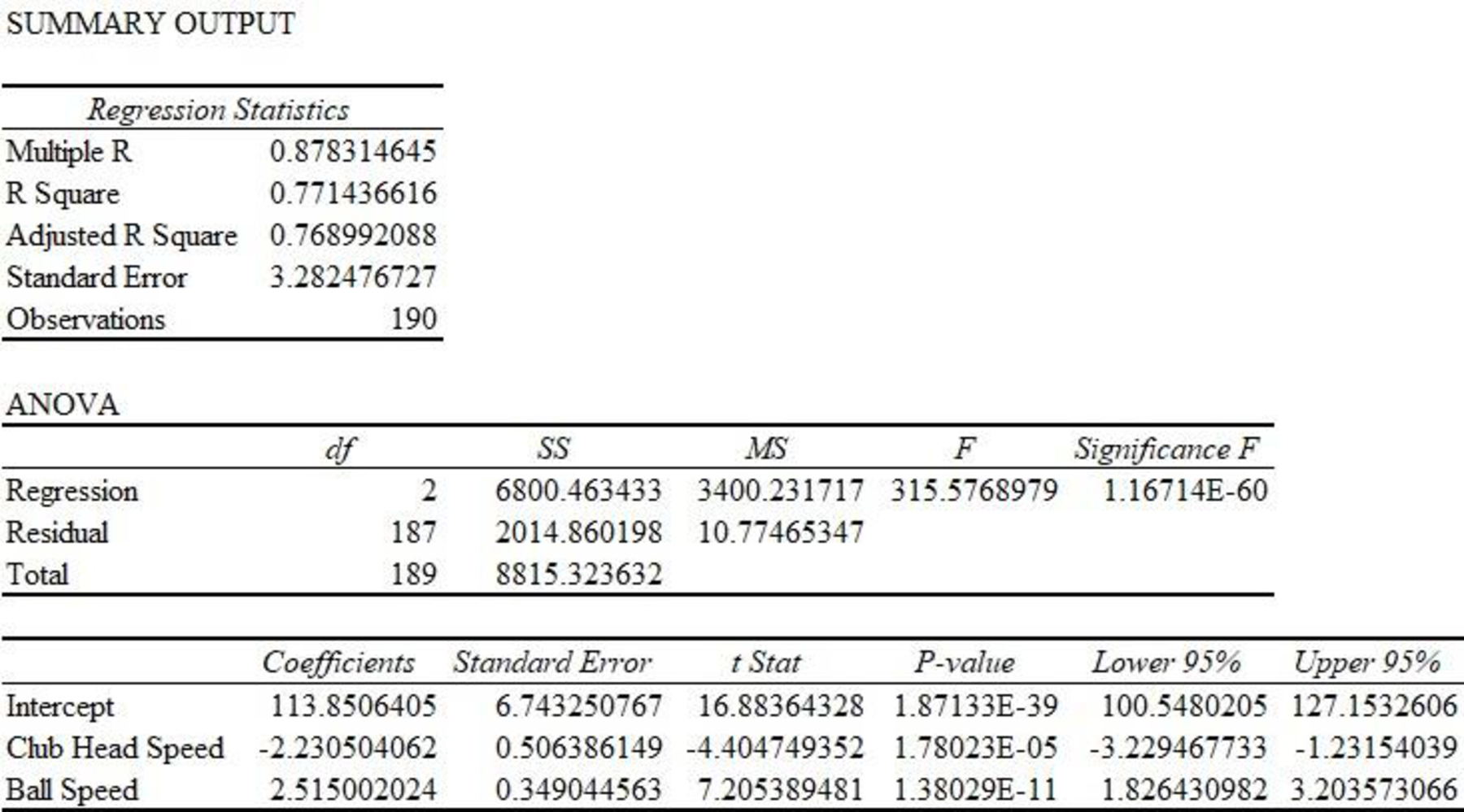
Thus, the estimated regression equation that could be used to predict the average number of yards per drive given both club head speed and ball speed is as follows:
In the given output,
Thus, only 77.14% variability in total distance can be explained by variability in club head and ball speed.
Scatter Diagram:
Software procedure:
Step-by-step procedure to obtain scatter diagram using EXCEL software:
- Open the file PGADrivingDist.
- Select the cell Range $B$1:$C$191.
- Go to insert and select scatter plot.
- Click OK
Output obtained using EXCEL software is given as follows:
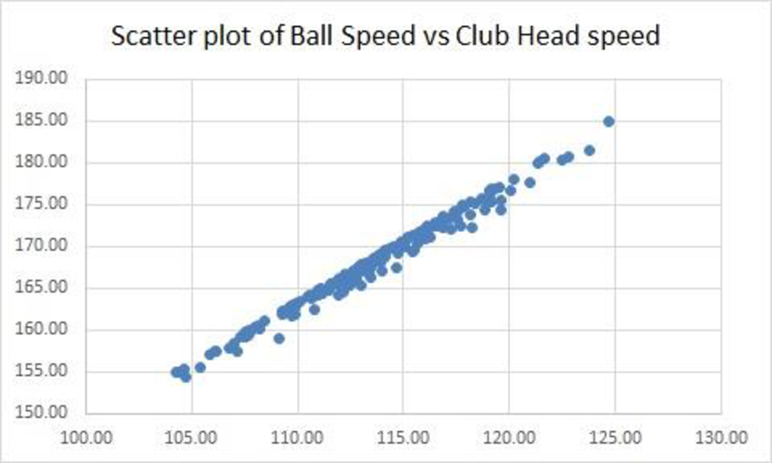
The scatter diagram exhibits a strong positive linear relationship between ball speed and club head speed. Both the variables in the same model are not recommended as the linear effect of one variable describes the linear effect of the other variable. As a result, the other variable will be of little additional value. Thus, there is a chance of multicollinearity.
Thus, developing an estimated regression equation that uses both club head speed and ball speed to predict the average number of yards per drive is not useful.
d.
Find the estimated regression equation that could be used to predict the average number of yards per drive given the ball speed and the launch angle.
Answer to Problem 9E
The estimated regression equation that could be used to predict the average number of yards per drive given both ball speed and launch angle is as follows:
Explanation of Solution
Calculation:
The regression equation can be obtained using Excel software.
Regression:
Software procedure:
Step-by-step procedure to get the regression equation using EXCEL software:
- Open the file PGADrivingDist.
- Select Data > Data Analysis > Regression.
- Click OK.
- Under Input Y Range enter $E$1:$E$191.
- Under Input X Range enter $C$1:$D$191.
- Click the box of Labels.
- Under Output Range enter $H$24.
- Click OK.
Output obtained using EXCEL software is given as follows:
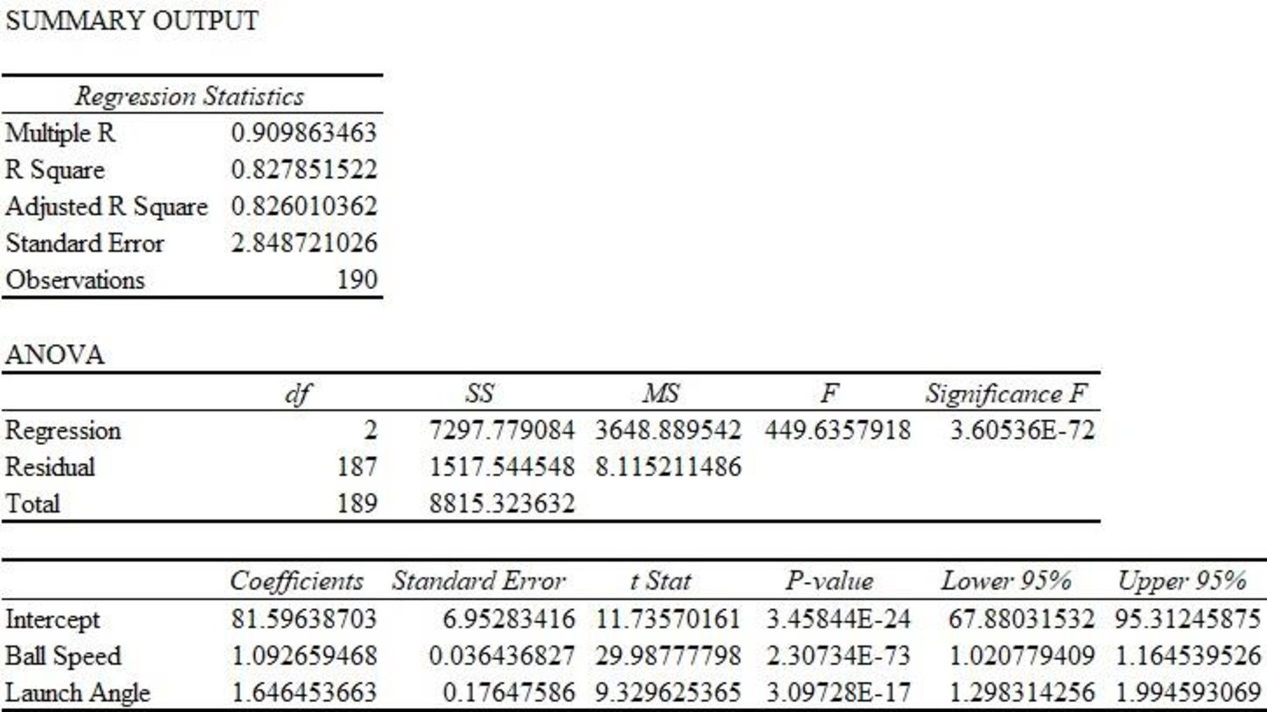
Thus, the estimated regression equation that could be used to predict the average number of yards per drive given both ball speed and launch angle is as follows:
e.
Predict the average number of yards per drive for the new player using the obtained equation in part (d).
Answer to Problem 9E
The predicted average number of yards per drive for the new player is 285.465 yards.
Explanation of Solution
Calculation:
The ball speed of a new PGA player is 170 mph with launch angle of 11 degrees.
From Part (b), it is found that the estimated regression equation that could be used to predict the average number of yards per drive given both club head speed and launch angle is
Thus, the predicted average number of yards per drive for the new player is as follows:
Thus, the predicted average number of yards per drive for the new player is 285.465 yards.
Want to see more full solutions like this?
Chapter 15 Solutions
Modern Business Statistics with Microsoft Office Excel (with XLSTAT Education Edition Printed Access Card)


- Question 1 The data shown in Table 1 are and R values for 24 samples of size n = 5 taken from a process producing bearings. The measurements are made on the inside diameter of the bearing, with only the last three decimals recorded (i.e., 34.5 should be 0.50345). Table 1: Bearing Diameter Data Sample Number I R Sample Number I R 1 34.5 3 13 35.4 8 2 34.2 4 14 34.0 6 3 31.6 4 15 37.1 5 4 31.5 4 16 34.9 7 5 35.0 5 17 33.5 4 6 34.1 6 18 31.7 3 7 32.6 4 19 34.0 8 8 33.8 3 20 35.1 9 34.8 7 21 33.7 2 10 33.6 8 22 32.8 1 11 31.9 3 23 33.5 3 12 38.6 9 24 34.2 2 (a) Set up and R charts on this process. Does the process seem to be in statistical control? If necessary, revise the trial control limits. [15 pts] (b) If specifications on this diameter are 0.5030±0.0010, find the percentage of nonconforming bearings pro- duced by this process. Assume that diameter is normally distributed. [10 pts] 1arrow_forward4. (5 pts) Conduct a chi-square contingency test (test of independence) to assess whether there is an association between the behavior of the elderly person (did not stop to talk, did stop to talk) and their likelihood of falling. Below, please state your null and alternative hypotheses, calculate your expected values and write them in the table, compute the test statistic, test the null by comparing your test statistic to the critical value in Table A (p. 713-714) of your textbook and/or estimating the P-value, and provide your conclusions in written form. Make sure to show your work. Did not stop walking to talk Stopped walking to talk Suffered a fall 12 11 Totals 23 Did not suffer a fall | 2 Totals 35 37 14 46 60 Tarrow_forwardQuestion 2 Parts manufactured by an injection molding process are subjected to a compressive strength test. Twenty samples of five parts each are collected, and the compressive strengths (in psi) are shown in Table 2. Table 2: Strength Data for Question 2 Sample Number x1 x2 23 x4 x5 R 1 83.0 2 88.6 78.3 78.8 3 85.7 75.8 84.3 81.2 78.7 75.7 77.0 71.0 84.2 81.0 79.1 7.3 80.2 17.6 75.2 80.4 10.4 4 80.8 74.4 82.5 74.1 75.7 77.5 8.4 5 83.4 78.4 82.6 78.2 78.9 80.3 5.2 File Preview 6 75.3 79.9 87.3 89.7 81.8 82.8 14.5 7 74.5 78.0 80.8 73.4 79.7 77.3 7.4 8 79.2 84.4 81.5 86.0 74.5 81.1 11.4 9 80.5 86.2 76.2 64.1 80.2 81.4 9.9 10 75.7 75.2 71.1 82.1 74.3 75.7 10.9 11 80.0 81.5 78.4 73.8 78.1 78.4 7.7 12 80.6 81.8 79.3 73.8 81.7 79.4 8.0 13 82.7 81.3 79.1 82.0 79.5 80.9 3.6 14 79.2 74.9 78.6 77.7 75.3 77.1 4.3 15 85.5 82.1 82.8 73.4 71.7 79.1 13.8 16 78.8 79.6 80.2 79.1 80.8 79.7 2.0 17 82.1 78.2 18 84.5 76.9 75.5 83.5 81.2 19 79.0 77.8 20 84.5 73.1 78.2 82.1 79.2 81.1 7.6 81.2 84.4 81.6 80.8…arrow_forward
- Name: Lab Time: Quiz 7 & 8 (Take Home) - due Wednesday, Feb. 26 Contingency Analysis (Ch. 9) In lab 5, part 3, you will create a mosaic plot and conducted a chi-square contingency test to evaluate whether elderly patients who did not stop walking to talk (vs. those who did stop) were more likely to suffer a fall in the next six months. I have tabulated the data below. Answer the questions below. Please show your calculations on this or a separate sheet. Did not stop walking to talk Stopped walking to talk Totals Suffered a fall Did not suffer a fall Totals 12 11 23 2 35 37 14 14 46 60 Quiz 7: 1. (2 pts) Compute the odds of falling for each group. Compute the odds ratio for those who did not stop walking vs. those who did stop walking. Interpret your result verbally.arrow_forwardSolve please and thank you!arrow_forward7. In a 2011 article, M. Radelet and G. Pierce reported a logistic prediction equation for the death penalty verdicts in North Carolina. Let Y denote whether a subject convicted of murder received the death penalty (1=yes), for the defendant's race h (h1, black; h = 2, white), victim's race i (i = 1, black; i = 2, white), and number of additional factors j (j = 0, 1, 2). For the model logit[P(Y = 1)] = a + ß₁₂ + By + B²², they reported = -5.26, D â BD = 0, BD = 0.17, BY = 0, BY = 0.91, B = 0, B = 2.02, B = 3.98. (a) Estimate the probability of receiving the death penalty for the group most likely to receive it. [4 pts] (b) If, instead, parameters used constraints 3D = BY = 35 = 0, report the esti- mates. [3 pts] h (c) If, instead, parameters used constraints Σ₁ = Σ₁ BY = Σ; B = 0, report the estimates. [3 pts] Hint the probabilities, odds and odds ratios do not change with constraints.arrow_forward
- Solve please and thank you!arrow_forwardSolve please and thank you!arrow_forwardQuestion 1:We want to evaluate the impact on the monetary economy for a company of two types of strategy (competitive strategy, cooperative strategy) adopted by buyers.Competitive strategy: strategy characterized by firm behavior aimed at obtaining concessions from the buyer.Cooperative strategy: a strategy based on a problem-solving negotiating attitude, with a high level of trust and cooperation.A random sample of 17 buyers took part in a negotiation experiment in which 9 buyers adopted the competitive strategy, and the other 8 the cooperative strategy. The savings obtained for each group of buyers are presented in the pdf that i sent: For this problem, we assume that the samples are random and come from two normal populations of unknown but equal variances.According to the theory, the average saving of buyers adopting a competitive strategy will be lower than that of buyers adopting a cooperative strategy.a) Specify the population identifications and the hypotheses H0 and H1…arrow_forward
- You assume that the annual incomes for certain workers are normal with a mean of $28,500 and a standard deviation of $2,400. What’s the chance that a randomly selected employee makes more than $30,000?What’s the chance that 36 randomly selected employees make more than $30,000, on average?arrow_forwardWhat’s the chance that a fair coin comes up heads more than 60 times when you toss it 100 times?arrow_forwardSuppose that you have a normal population of quiz scores with mean 40 and standard deviation 10. Select a random sample of 40. What’s the chance that the mean of the quiz scores won’t exceed 45?Select one individual from the population. What’s the chance that his/her quiz score won’t exceed 45?arrow_forward
 Elementary Geometry For College Students, 7eGeometryISBN:9781337614085Author:Alexander, Daniel C.; Koeberlein, Geralyn M.Publisher:Cengage,
 Glencoe Algebra 1, Student Edition, 9780079039897...AlgebraISBN:9780079039897Author:CarterPublisher:McGraw Hill
 Holt Mcdougal Larson Pre-algebra: Student Edition...AlgebraISBN:9780547587776Author:HOLT MCDOUGALPublisher:HOLT MCDOUGAL