
Concept explainers
(a)
Calculate the Fourier transform of the function shown in the given Figure.
(a)
Answer to Problem 1P
The Fourier transform for the function given in Figure is
Explanation of Solution
Given data:
Refer to Figure given in the textbook.
Formula used:
Write the general expression for the function
Write the general expression for definite integral
Calculation:
In the given Figure, the function
The end points of the function
The slope of the straight line is calculated as follows,
Substitute
Therefore, for the given Figure, the function
Applying equation (3) in equation (2) as follows,
Consider,
Write the general expression for integration by parts method as follows,
By applying integration by parts to equation (5),
Applying equation (6) in equation (5) as follows,
Consider,
Consider,
Substitute
Substitute equation (9) in equation (7) as follows,
The above equation as follows,
Substitute equation (10) in equation (4), and applying the limits as follows,
Conclusion:
Thus, the Fourier transform for the function given in Figure is
(b)
Calculate
(b)
Answer to Problem 1P
The function
Explanation of Solution
Given data:
Refer to Part (a).
Formula used:
Write the general expression for L’Hospital’s rule as follows,
Calculation:
Applying equation (12) to equation (11) when
The above equation becomes,
Conclusion:
Thus, the function
(c)
Plot
(c)
Answer to Problem 1P
The sketch for
Explanation of Solution
Given data:
Refer to Part (a),
Calculation:
Appling
Create a table as shown in below Table 1.
Table 1
| Angular Frequency | Function |
| –200 | 0.0785 |
| –190 | 0.1041 |
| –180 | 0.1063 |
| –170 | 0.0819 |
| –160 | 0.0336 |
| –150 | 0.0295 |
| –140 | 0.0943 |
| –130 | 0.1452 |
| –120 | 0.1678 |
| –110 | 0.1522 |
| –100 | 0.0951 |
| –90 | 0.0014 |
| –80 | 0.1161 |
| –70 | 0.2389 |
| –60 | 0.3457 |
| –50 | 0.4162 |
| –40 | 0.4354 |
| –30 | 0.3962 |
| –35 | 0.3012 |
| –15 | 0.1625 |
| 0 | 5.0000 (Original value is infinity, though for the instance consider one finite value as 5) |
| 10 | 0.1625 |
| 20 | 0.3012 |
| 30 | 0.3962 |
| 40 | 0.4354 |
| 50 | 0.4162 |
| 60 | 0.3457 |
| 70 | 0.2389 |
| 80 | 0.1161 |
| 90 | 0.0014 |
| 100 | 0.0951 |
| 110 | 0.1522 |
| 120 | 0.1678 |
| 130 | 0.1452 |
| 140 | 0.0943 |
| 150 | 0.0295 |
| 160 | 0.0336 |
| 170 | 0.0819 |
| 180 | 0.1063 |
| 190 | 0.1041 |
| 200 | 0.0785 |
Sketch the plot for various values of function
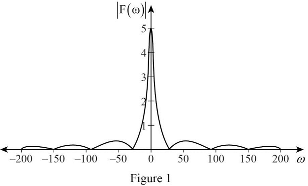
Conclusion:
Thus, the sketch for
Want to see more full solutions like this?
Chapter 17 Solutions
ELECTRIC CIRCUITS& INTR. TO PSPIC W/MAS


 Introductory Circuit Analysis (13th Edition)Electrical EngineeringISBN:9780133923605Author:Robert L. BoylestadPublisher:PEARSON
 Delmar's Standard Textbook Of ElectricityElectrical EngineeringISBN:9781337900348Author:Stephen L. HermanPublisher:Cengage Learning
 Programmable Logic ControllersElectrical EngineeringISBN:9780073373843Author:Frank D. PetruzellaPublisher:McGraw-Hill Education
 Fundamentals of Electric CircuitsElectrical EngineeringISBN:9780078028229Author:Charles K Alexander, Matthew SadikuPublisher:McGraw-Hill Education
 Electric Circuits. (11th Edition)Electrical EngineeringISBN:9780134746968Author:James W. Nilsson, Susan RiedelPublisher:PEARSON
 Engineering ElectromagneticsElectrical EngineeringISBN:9780078028151Author:Hayt, William H. (william Hart), Jr, BUCK, John A.Publisher:Mcgraw-hill Education,