
Videos
The business problem facing a consumer products company is to measures the effectiveness of difference types of advertising media in the promotion of its products. Specifically, the company is interested in the effectiveness of ratio advertising and newspaper advertising (including the cost of discount coupons). During a one-month test period, data were collected from a sample of 22 cities with approximately equal populations. Each city is allocated a specific expenditure level for radio advertising and for newspaper advertising. The sales of the product (in thousands of dollars) and also the levels of media expenditure (in thousands of dollars) during the test month are recorded and stored a Advertise.
a. Using all the data as the training sample, develop a regression tree model to predict the sales of the product.
b. What conclusions can you reach about the sales of the product?
a.
Develop a regression tree model to predict the sales of product.
Explanation of Solution
Use JMP to develop a regression tree model.
Software procedure:
Step by step by procedure to develop regression tree is given below:
Open Advertise file in JMP.
Select Analyze > Predictive Modelling > Partition.
Drag Sales to the Y, Response box.
Drag Radio to the X, Factor box.
Drag Newspaper to the X, Factor box.
Click Ok.
Click Split. Repeat this step until clicking Split no longer has any effect on the tree diagram.
The JMP result is shown below:
b.
Write conclusion about the sales of product.
Explanation of Solution
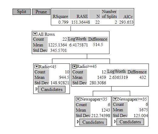
The tree model contains two splits and an
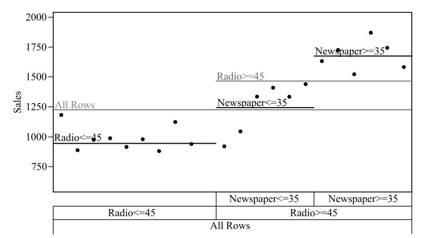
At the root node, the data has been split based on whether the radio expenditure is less than 45000 dollars or not. The subset less than 45000 dollars has a count of 10 cities with mean sales of 944.5 thousand dollars, which is less than the other subset having a count of 12 cities with mean 1459 thousand dollars.
The subset radio expenditure greater than 45000 dollars has been further split into two based on whether the newspaper expenditure is less than 35000 dollars or not and each further split has a count of 6 cities. The mean sales of newspaper expenditure less than 35000 dollars is less than the newspaper expenditure of 35000 or more.
Want to see more full solutions like this?
Chapter 17 Solutions
BASIC BUSINESS STATISTICS


- Urban Travel Times Population of cities and driving times are related, as shown in the accompanying table, which shows the 1960 population N, in thousands, for several cities, together with the average time T, in minutes, sent by residents driving to work. City Population N Driving time T Los Angeles 6489 16.8 Pittsburgh 1804 12.6 Washington 1808 14.3 Hutchinson 38 6.1 Nashville 347 10.8 Tallahassee 48 7.3 An analysis of these data, along with data from 17 other cities in the United States and Canada, led to a power model of average driving time as a function of population. a Construct a power model of driving time in minutes as a function of population measured in thousands b Is average driving time in Pittsburgh more or less than would be expected from its population? c If you wish to move to a smaller city to reduce your average driving time to work by 25, how much smaller should the city be?arrow_forwardA research group is interested in the relationship between exposure to mold in households after a major hurricane and the onset of acute respiratory illness in children. Suppose an observational study is conducted over 10 years following the natural disaster and the following two-by-two table was created in order to address the relationship between exposure and outcome. Acute Respiratory Illness No Acute Respiratory Illness Total Mold 378 156 534 No Mold 73 260 333 Total 451 416 867 Calculate the incidence of acute respiratory illness in the exposed and unexposed. Calculate the relative risk for ARI due to exposure in this study Interpret your findings from part Barrow_forwardThe director of student services at San Bernardino Valley College is interested in whether women are more likely to attend orientation than men before they begin their coursework. A random sample of freshmen at San Bernardino Valley College were asked to specify their gender and whether they attended the orientation. The results of the survey are shown below: Data for Gender vs. Orientation Attendance Women Men Yes 375 336 No 316 329 Let p1p1 be the proportion of women who attended the orientation and p2p2 be the proportion of men who attended the orientation. What can be concluded at the αα = 0.10 level of significance? What is the test statistic and p valuearrow_forward
- The management of BCD Inc. would like to separate the fixed and variable components of electricity as measured against machine hours in one of its plants. Data collected over the most recent six months follow:Electricity MachineMonth Cost Hours January $1,100 4,500February 1,110 4,700March 1,050 4,100April 1,200 5,000May 1,060 4,000June 1,120 4,600Required: 1. Using the method of least squares, compute the fixed cost and the variable cost rate for electricity expense. (Round estimates to the nearest cent.) 2. Compute coefficients of correlation and determinationarrow_forwardSuppose that weights of college mathematics textbooks in the United States are normally distributed with mean µ = 1.25 lbs and variance σ2 = 0.25 lb2. Find the weight that corresponds to Q1 and interpret this measure of position in the context of the problem.arrow_forwardA researcher wishes to study the relationship between education and income separately for individuals who have college degrees, and for those who don't. To this end, he interviews 100 individuals in each category. Survey results are listed in the table below. non college graduates college graduates avg education 13 yr 18 yr std. dev. education 2 yr 1.2 yr Sxx 396 yr2 143 yr2 Avg. Income $67,200 $84,950 std. dev. income $9,400 $10,500 correlation coefficient .25 .15 a. Use the data above to find point estimates for regression coefficients B0NG and B1NG for non-college graduates and BoG and B1G for college graduates. b. Propose an unbiased estimator for the difference theta=B1G - B1NG in slope coefficients for the two sub-populations, and show that B(theta hat)= 0. c. Assume that the error terms ENG and EG for non-graduates and graduates, respectively, are both distributed normally, with known standard deviation oENG = oEG = $ 10,000. In that case, determine the…arrow_forward
- What is the step-step solution to this problem? Does posting calorie content for menu items affect people’s choices in fast-food restaurants? According to results obtained by Elbel, Gyamfi, and Kersh (2011), the answer is no. The researchers monitored the calorie content of food purchases for children and adolescents in four large fast-food chains before and after mandatory labeling began in New York City. Although most of the adolescents reported noticing the calorie labels, apparently the labels had no effect on their choices. Data similar to the results obtained show an average of M = 786 calories per meal with s = 85 for n = 100 children and adolescents before the labeling, compared to an average of M = 772 calories with s = 91 for a similar sample of n = 100 after the mandatory posting. Use a two-tailed test with a α .05 to determine whether the mean number of calories after the posting is significantly different than before calorie content was posted. 3. Calculate r 2 to…arrow_forwardSuppose that weights of college mathematics textbooks in the United States are normally distributed with mean µ = 2.25 lbs and variance σ2 = 0.2025 lbs. Find the weight that corresponds to Q3 and interpret this measure of position in the context of the problem.arrow_forwardThe staff of controller of McCourt Company added the variable "pounds moved" to the ten-month data set: Month Materials Handling Cost Number of Moves Pounds Moved January $5,600 475 12,000 February 3,090 125 15,000 March 2,780 175 7,800 April 8,000 600 29,000 May 1,990 200 600 June 5,300 300 23,000 July 4,300 250 17,000 August 6,300 400 25,000 September 2,000 100 6,000 October 6,240 425 22,400 Required: 1. Using the data on material handling, use regression software such as Microsoft Excel to complete the missing data in the table below (round regression parameters to the nearest cent and other answers to three decimal places): McCourt CompanySUMMARY OUTPUT Regression Statistics Multiple R 0.999 R Square fill in the blank 491c8af8afe4f84_1 Adjusted R Square fill in the blank 491c8af8afe4f84_2 Standard Error 119.600 Observations 10 ANOVA df SS MS F Significance F Regression 2 37,768,070.16 18,884,035…arrow_forward
 Functions and Change: A Modeling Approach to Coll...AlgebraISBN:9781337111348Author:Bruce Crauder, Benny Evans, Alan NoellPublisher:Cengage Learning
 Glencoe Algebra 1, Student Edition, 9780079039897...AlgebraISBN:9780079039897Author:CarterPublisher:McGraw Hill