
Videos
a.
Determine the typical seasonal patterns for sales using the ratio-to-moving-average method.
a.
Answer to Problem 28CE
The typical seasonal patterns for sales are 1.191168, 1.121778, 0.435094 and 1.251959, respectively.
Explanation of Solution
Calculation:
Four-Year moving average:
Centered Moving Average:
Specific seasonal index:
| Year | Quarter | Visitors |
Four-quarter moving average |
Centered Moving average | Specific seasonal |
| 2010 | 1 | 210 | |||
| 2 | 180 | ||||
| 3 | 60 | 174.5 | 0.34384 | ||
| 4 | 246 | 174 | 179.5 | 1.370474 | |
| 2011 | 1 | 214 | 175 | 186.75 | 1.145917 |
| 2 | 216 | 184 | 187.5 | 1.152 | |
| 3 | 82 | 189.5 | 189.5 | 0.432718 | |
| 4 | 230 | 185.5 | 195 | 1.179487 | |
| 2012 | 1 | 246 | 193.5 | 197.625 | 1.244782 |
| 2 | 228 | 196.5 | 205 | 1.112195 | |
| 3 | 91 | 198.75 | 212.75 | 0.427732 | |
| 4 | 280 | 211.25 | 217 | 1.290323 | |
| 2013 | 1 | 258 | 214.25 | 222.5 | 1.159551 |
| 2 | 250 | 219.75 | 227.5 | 1.098901 | |
| 3 | 113 | 225.25 | 232.375 | 0.486283 | |
| 4 | 298 | 229.75 | 237.125 | 1.256721 | |
| 2014 | 1 | 279 | 235 | 239.625 | 1.164319 |
| 2 | 267 | 239.25 | 240.75 | 1.109034 | |
| 3 | 116 | 240 | 244.375 | 0.47468 | |
| 4 | 304 | 241.5 | 250.125 | 1.215392 | |
| 2015 | 1 | 302 | 247.25 | 252.75 | 1.194857 |
| 2 | 290 | 253 | 253.25 | 1.145114 | |
| 3 | 114 | 252.5 | 256.375 | 0.444661 | |
| 4 | 310 | 254 | 258.875 | 1.197489 | |
| 2016 | 1 | 321 | 258.75 | 259.75 | 1.235804 |
| 2 | 291 | 259 | 261.75 | 1.111748 | |
| 3 | 120 | 260.5 | |||
| 4 | 320 | 263 |
The Quarterly indexes are,
| I | II | III | IV | |
| 2010 | 0.34384 | 1.370474 | ||
| 2011 | 1.145917 | 1.152 | 0.432718 | 1.179487 |
| 2012 | 1.244782 | 1.112195 | 0.427732 | 1.290323 |
| 2013 | 1.159551 | 1.098901 | 0.486283 | 1.256721 |
| 2014 | 1.164319 | 1.109034 | 0.47468 | 1.215392 |
| 2015 | 1.194857 | 1.145114 | 0.444661 | 1.197489 |
| 2016 | 1.235804 | 1.111748 | ||
| Mean | 1.190871 | 1.121499 | 0.434986 | 1.251648 |
Typical Seasonal index:
Here,
Therefore,
The seasonal indexes are,
| I | II | III | IV | |
| 2010 | 0.34384 | 1.370474 | ||
| 2011 | 1.145917 | 1.152 | 0.432718 | 1.179487 |
| 2012 | 1.244782 | 1.112195 | 0.427732 | 1.290323 |
| 2013 | 1.159551 | 1.098901 | 0.486283 | 1.256721 |
| 2014 | 1.164319 | 1.109034 | 0.47468 | 1.215392 |
| 2015 | 1.194857 | 1.145114 | 0.444661 | 1.197489 |
| 2016 | 1.235804 | 1.111748 | ||
| Mean | 1.190871 | 1.121499 | 0.434986 | 1.251648 |
| Typical Seasonal Index | 1.191168 | 1.121778 | 0.435094 | 1.251959 |
b.
Determine the trend equation.
b.
Answer to Problem 28CE
The trend equation is
Explanation of Solution
Calculation:
Deseasonalization:
| Sales | Typical seasonal index | Deseasonalized Sales |
| 210 | 1.191168 | 176.29755 |
| 180 | 1.121778 | 160.4595562 |
| 60 | 0.435094 | 137.9012351 |
| 246 | 1.251959 | 196.4920576 |
| 214 | 1.191168 | 179.6555985 |
| 216 | 1.121778 | 192.5514674 |
| 82 | 0.435094 | 188.4650214 |
| 230 | 1.251959 | 183.7120864 |
| 246 | 1.191168 | 206.5199871 |
| 228 | 1.121778 | 203.2487711 |
| 91 | 0.435094 | 209.1502066 |
| 280 | 1.251959 | 223.6494965 |
| 258 | 1.191168 | 216.5941328 |
| 250 | 1.121778 | 222.8604947 |
| 113 | 0.435094 | 259.7139928 |
| 298 | 1.251959 | 238.0269641 |
| 279 | 1.191168 | 234.2238878 |
| 267 | 1.121778 | 238.0150083 |
| 116 | 0.435094 | 266.6090546 |
| 304 | 1.251959 | 242.8194534 |
| 302 | 1.191168 | 253.5326671 |
| 290 | 1.121778 | 258.5181738 |
| 114 | 0.435094 | 262.0123468 |
| 310 | 1.251959 | 247.6119426 |
| 321 | 1.191168 | 269.4833978 |
| 291 | 1.121778 | 259.4096158 |
| 120 | 0.435094 | 275.8024703 |
| 320 | 1.251959 | 255.5994246 |
Assign t value as 1 for first quarter of 2010, 2 for the second quarter of 2011 and so on.
Step-by-step procedure to obtain the regression using the Excel:
- Enter the data for Sales and t in Excel sheet.
- Go to Data Menu.
- Click on Data Analysis.
- Select ‘Regression’ and click on ‘OK’
- Select the column of Deseasonalized Sales under ‘Input Y
Range ’. - Select the column of t under ‘Input X Range’.
- Click on ‘OK’.
Output for the Regression obtained using the Excel is as follows:
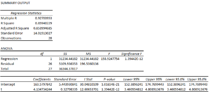
From the Excel output, the regression equation is
c.
Project the sales for the four quarters of next year using the trend equation.
Find the seasonally adjusted values.
c.
Answer to Problem 28CE
The sales for the four quarters for next year are 283.487, 287.6217, 291.7564 and 295.8911.
The seasonally adjusted values are 337.6806, 322.6477, 126.9415 and 370.4435.
Explanation of Solution
Calculation:
From the output, the regression equation is
The t value for first quarter of 2017 is 29.
The t value for second quarter of 2017 is 30.
The t value for third quarter of 2017 is 31.
The t value for fourth quarter of 2017 is 32.
Seasonally Adjusted Forecast:
| Estimated Visitors | Seasonal Index | |
| 283.487 | 1.191168 | 337.6806 |
| 287.6217 | 1.121778 | 322.6477 |
| 291.7564 | 0.435094 | 126.9415 |
| 295.8911 | 1.251959 | 370.4435 |
Want to see more full solutions like this?
Chapter 18 Solutions
STATISTICAL TECHNIQUES...LL >CUSTOM<


 Glencoe Algebra 1, Student Edition, 9780079039897...AlgebraISBN:9780079039897Author:CarterPublisher:McGraw Hill
 Big Ideas Math A Bridge To Success Algebra 1: Stu...AlgebraISBN:9781680331141Author:HOUGHTON MIFFLIN HARCOURTPublisher:Houghton Mifflin Harcourt
 Holt Mcdougal Larson Pre-algebra: Student Edition...AlgebraISBN:9780547587776Author:HOLT MCDOUGALPublisher:HOLT MCDOUGAL